Parallel computing has become a practical approach to industrial modeling. It brings formerly insoluble problems into solution range and makes formerly difficult-to-solve problems routine. The software challenges for the development of industrial quality codes for parallel computers, however, are great. In this book, we provide in-depth case studies of seventeen applications that were either re-designed or designed from scratch to solve industrial strength problems on parallel computers. We document both the solution process and the resulting performance of the application software. Additionally, we provide an overview of the terminology, basic hardware, performance issues, programming models, software tools, and other details that are necessary for researchers and students to become able parallel programmers. Finally, we show how, for industry to continue to participate in the parallel-computing arena, the applications must be portable and tailored to accommodate a rapidly changing hardware environment.
Parallel computing became a significant subfield of computer science by the late 1960's, but only by the late 1980's had hardware and software technology improved sufficiently for parallel computing to affect the day-to-day lives of applications programmers. As such, it spurred the development of a whole new way of thinking about programming for applications. Rather than deal with the old textbook picture of a flow-charted program going from one step to the next in a sequential fashion, the availability of parallel computers has forced us to rethink our algorithms at every step to determine which tasks can be performed independently and simultaneously with others. In the early days of parallel computing, this transition to parallel algorithms and the associated tools and programming languages remained primary in the research and university setting. As introduction of massively parallel computers based on workstation or commodity chips surfaced, however, these machines that are capable of gigaflop performance and terabyte data storage enticed industry into the growing field of parallel computing. Parallel computing is no longer confined to the research arena. The term massively parallel architecture even entered (with definitions provided) into popular magazines such as "Time" and "Parade" when a parallel computer designed by IBM was finally able to defeat the world chess champion Gary Kasparov in 1997. This parallel machine's calculating speed, which was doubled that year, can analyze 200 million possible moves per second--50 billion board positions in the three minutes given for each move.
In industry, parallel computers provide application-specific solutions to concurrent problems in today's market place. For the industrial participant, the challenge is to retool their computational modeling to harness the cost effectiveness of parallel high-performance computer systems in a way that is not possible with general purpose computers. This book presents a set of real experiences in porting useful applications to parallel computers. A majority of the applications discussed in this book were the result of collaboration between researchers at universities and national laboratories and their counterparts in industrial settings. The collaborations were spawned as part of an outreach program of Cray Research to help industrial customers re-tool their computer scientists to develop industrial strength software that would perform on the Cray T3D and Cray T3E massively parallel computer systems. This outreach program involved researchers at various institutes in the United States and Europe and was coined the Parallel Applications Technology Program (PATP).
This book focuses on tools and techniques for parallelizing scientific and technical applications in a lessons-learned fashion based on the experiences of researchers active in the field of applied parallel computing. In the introductory material, we provide
This is followed by detailed case studies of seventeen applications giving problem background, their approach to parallel solution, and performance results. In the final part of the book, we summarize results and lessons learned from the applications, give advice on designing industrial applications, and discuss our view of the future of industrial parallel computing. A glossary is included for defining terms in the book including the application chapters.
Industrial strength applications have been driving supercomputer architectures for many years. Each year a new machine design appears on the horizon, and with the availability of that new machine the door is open to the applications scientist. The question must be asked--can my application benefit from this new architecture? What speed-up is possible? What effort is necessary to port or design a code for this new computer? Fortunately, there is somewhat of a convergence in architectures for the very reason that ultimately, once the decision is made to split a problem up into parallel tasks, there are only a few basic principals that must be understood. In the next sections, we give the reader the appropriate terminology to understand all of the current parallel platforms, and presumably these same concepts will be essential in future designs. This material is at the introductory level, and provides the necessary foundation for understanding the terminology and techniques used in the applications chapters.
One of the hardest problems to overcome when getting started in a new field, and this is particularly true of computing fields, is the acronym terminology that prevails. Even at the onset, parallel computing used a wide variety of acronyms. Additionally, due to the rapid pace at which computer architecture is developing, newer architectures do not always fit well into categories that were invented before the architecture was. Historically, the most common classification scheme for parallel computers (due to Flynn) is based on a 4-letter mnemonic where the first two letters pertain to instructions that act on the data and the second two letters refer to the data stream type[Fin72]. These are:
A diagram showing the basic difference between the MIMD-SM and MIMD-DM is given in Figure 1. Another possible programming model is based on the parallel SIMD approach, whereby all processors are controlled to execute in a lock-step fashion. This parallel SIMD approach is too restrictive for the applications considered in this book. In the figure, CPU stands for central processing unit. Note that the SIMD computers do not have CPUs, they have Processing Elements (PEs). The difference is that a CPU fetches its own instructions and has its own program counter that points to the instruction to be fetched at a given instant. A processing element is fed instructions by its control unit, which has the single program counter.
Figure 1. The basic differences between the MIMD-SM, MIMD-DM, and (parallel) SIMD. For simplicity, we class MIMD-DM as MPP. DMP, for Distributed Memory Parallel is also used for MIMD-DM.
Adding to the terminology confusion, we have SPMD, which stands for Single Program Multiple Data and is basically a restriction of the MIMD model. In SPMD, each processor executes exactly the same program on a different subset of the program data. Every data item in the program is allocated to one processor and often every processor is allocated approximately equal numbers of data items. In practice, however, even with the SPMD model, the programmer can designate a master processor by judicious use of conditional statements. While some of this terminology is being replaced by a smaller set of acronyms described in the next section, (e.g., MIMD-DM becomes simply MPP) it is still found and referred to both in the papers in this book and throughout the literature.
Since Flynn introduced the taxonomy (his paper written in 1969-70 and published in 1972), computers have been advancing at an enormous rate. Yet, the terminology persists and is referred to in many of the applications chapters. One problem is where to classify the first (single processor) vector architectures such as the Cray-1 and the NEC SX-1. There is some disagreement as to whether these machines should be classified as SIMD or SISD. The agruments for using the SIMD classification are that a single instruction operates on many datum and the programming considerations for performance (i.e., data independance, concurrency) are the same for vectorization as they are for machines like the CM2. The arguments for the SISD classification are that the execution of the operations happens in a pipelined fashion and that modern microprocessors (like those appearing on the desktop and classified as SISD) are starting to incorporate vector instructions. Since this point is somewhat controversial, whereever possible we avoid using the Flynn Taxonomy except for historical references. Finally, vector machines with shared memory and multiple processors such as the Cray XMP and the Cray C90 are referred to as PVP for Parallel Vector Platform.
The programs described in this book are written primarily for the MIMD-DM class of computers, which includes the Cray T3D and T3E and the IBM SP parallel systems. We use the term MPP (massively parallel processing) for this class of computers. When the projects described in the applications chapters were initiated in the mid-1990's the MPP architecture was one of the most difficult of the current high-performance supercomputing architectures to design codes for. This was due not only to the purely distributed memory, which caused the programmer to totally rethink a problem's implementation, but is also due to the initial lag in the development and availability of parallel tools and programming standards for the MPP machines. Thus, it took a while before the MPP paradigm made its way into general industrial computing. The application chapters of the book detail the case histories of several large scientific and industrial applications, which successfully made the jump to the MPP platform. However, since they are large industrial applications, they cannot afford to be written to perform on one type of architecture alone. They must be written to withstand the continual upgrade and redesign of computer architectures. There is still a contention in the field of supercomputing as to which of the architectures will ultimately win the price/performance race. In fact, as this book is being written, architectures are once again undergoing a transformation. Some of the current "hottest architectures" being built now exploit a hybrid of the shared memory and distributed memory thus requiring even more complex programming models.
The high performance computers available today generally fall into one of three major classes, the SMP, the MPP, and the NUMA generalization of the SMP. The term SMP originated to mean a symmetric multiprocessor, referring to the uniform way in which the processors are often connected to the shared memory. But as Culler points out, the widely-used term SMP causes some confusion [Cul98]. The major design issue in an SMP is that all processors have equal access to the shared resources, namely shared memory and I/O functionality. The time for a processor to access the memory should be the same for all processors. As Culler states, even if the location is cached, the access will still be symmetric with respect to the processors. (Part of the confusion here is the occasional use of SMP to refer to "shared memory parallel." Following this same line of thinking, the MPP architecture may simply be referred to as a member of the DMP or "distributed memory parallel" class.) The MPP systems originated as a straightforward generalization in which fast workstations or personal computers are connected, which themselves are based on RISC (Reduced Instruction Set Computer) microprocessors. For the simplest description of an MPP computer, one can partition it into processors, memory with various access levels including cache(s), interconnect network or switch, and support hardware. (See Figure 2.) Some details of these various components of an MPP computer are discussed in the following subsections.
Figure 2. Typical specifications of MIMD-DM or MPP computers.
The most powerful systems in use by industry today are the SMP and the MPP. In the classic MPP, the memory is truly distinct (and thus the performance is also very scalable). In the SMP, the processors share a global area of RAM (memory). The purpose of such architecture is to avoid some of the problems associated with interprocessor communication. However, the shared RAM design of the SMP can lead to bottlenecks as more and more processors are added, i.e., a bus or switch used to access the memory may become overloaded. Thus, the SMP systems do not share the same potential for scalability as their MPP cousins. One way to avoid the scalability problems on the SMP is the re-introduction of non-uniform memory access or NUMA into the system. NUMA a dds other levels of memory, shared among a subset of processors, that can be accessed without using the bus-based network. This further generalization of the SMP architecture is an attempt to regain some of the scalability lost by offering shared memory. Vendors have come to coin these architectures as ccNUMA, using cc to stress that cache coherency (see below) is retained as multiple SMP nodes are linked by a cache coherent interconnect.
Caches are becoming more important because processor speeds are increasing much faster than memory access speeds. A read or write to cache generally requires less than 10 processor clock periods as compared to 100 clock periods or more to access normal memory. However, the basic problem with using caches is that multiple copies of data can exist. Significant effort at the hardware and software levels is required to insure that all processors use the latest data. This requirement is referred to as cache coherency. The use of caches is discussed in more detail in section 2.2.2.
One of the latest developments in high performance computing is the coupling of SMP machines into clusters using very high speed interconnects. These clusters can have total number of processors that are comparable to large MPP machines. A typical cluster configuration is shown in Figure 3. They present the application developer the benefit of relatively large shared memory within a given SMP and total memory comparable to MPP machines. The clustering concept is not restricted to joining SMPs, many architectures are suitable for nodes of a cluster, and the nodes need not necessarily be all of the same type. This is often referred to as a "convergence of architectures" in the development of high-end computing.
Figure 3. Example of a cluster of SMPs or symmetric multiprocessors such as the DEC Alpha. Here the single letter C denotes cache.
To use entire clusters effectively the developer must divide the problem into levels of parallelism and often needs to use a combination of the programming models discussed in Section 4. One advantage of clusters is that they are designed to allow computer centers to add additional nodes as needed given the economic driving force. Typical SMPs available now as a cluster can be RISC based or vector based. The NEC SX-4 system is a recent example of a vector-based SMP than can be configured into a cluster. A single SX-4 SMP or node can have 4 to 32 processors and the cluster can have 2 to 16 nodes. The nodes are connected with a fiber-optic non-blocking crossbar having an 8 GB/s bi-directional bandwidth. For such vector machines there are now three levels of parallelism, namely distributed memory parallelism across the nodes, shared-memory parallelism within the nodes, and finally, vector parallelism associated with the vector units. For each of the levels of parallelism a different programming model (see Section 4) may be the appropriate choice, leading to additional complexity and challenges for programming. In order to distinguish these new clusters from clusters of workstations, the later are generally referred to as NOWs (Network of Workstations). While the processor count for NOWs can be large, the first implementations of this architecture had slow communication speed that limited them to problems that required very small amount of communication compared to processor usage. As technology advances, improved communication speed and the ease at which these systems can be created. (See e.g., "How to build a Beowulf.")
Ultimately all systems contain some level of similarity in the mind of the applications programmers, because for example, even memory that is logically shared is still physically distributed on today's parallel machines. Breaking the problem into appropriate tasks is fundamental to all parallel architectures, and doing so in an architecture independent manner helps to promote the longevity of a particular application code.
The reason that parallel computers have become a viable means of performing large industrial scale calculations is the same reason that every business and home has easy access to personal computing--the RISC-processor technology for fast and efficient chips combined with manufacturing improvements to shrink the geometry has made commodity processors very inexpensive. Parallel machines today consist of either off-the-shelf chips, or in certain cases, chips that have been modified from the off-the-shelf version to include additional caches and other support structure to ideally suit them for being combined together into a large parallel computer. For example, in the case of the Cray T3D and T3E line of architectures, the chip is formed using low-cost CMOS technology (based on a Metal Oxide Semiconductor). The result is an extremely fast RISC-based microprocessor (manufactured by Digital Equipment Corporation) called the Alpha EV4 (150 or 200 MHz) in the Cray T3D and the EV5 in the Cray T3E. Initial shipments of the EV5 chip give it a peak performance of 600 million floating point operations per second (megaflops or MFlops) in IEEE standard 32-bit and 64-bit mode running at a speed of 300 MHz. Continual upgrades of the chip increased the speed to 450, and finally 600 MHz by 1997. In some instances, the chips implemented in the MPPs run about one year behind their implementation in workstations, since the MPP support must be compatible with the new chip.
Another dominant player in the MPP arena is the IBM RS/6000 SP. The SP series is available in configurations that we informally term as "standard" or "hybrid" where the standard configuration has one processor per node and the hybrid versions have an SMP on each node. The earlier SP machines were based on the 66 MHz POWER2 processors arranged in a standard configuration. By 1995 according to IDC (International Data Corporation), the IBM RS/6000 SP was the best selling MPP system in Europe. In 1996 the P2SC technology was introduced, which integrated eight POWER2 chips into a single POWER2 Super Chip which at 120 MHz is capable of 480 MFlops peak performance. This has been followed by P2SC processors running at 160 MHz and rated at 640 MFlops peak performance. The carefully balanced architecture of these P2SC processors allows them to obtain high levels of performance on a wide variety of scientific and technical applications. In the class of "hybrid" configurations, a recent SP version has a 4-way SMP on each node with each PowerPC 604e processor in the node running at 332 MHz leading to a peak performance rating of 2.656 GFlops per node (since each processor can perform two floating point operations per cycle). Two of these machines have been placed at the Lawrence Livermore National Laboratories as part of the U.S. government's Advanced Strategic Computing Initiative (ASCI). Each of these machines has 168 nodes with four 332 MHz PowerPC 604e processors sharing memory on each node; one of them has additional POWER2 Nodes. A larger machine with 1464 nodes and 4 processors per node is currently in the installation process. In Figure 4, we show a greatly simplified schematic diagram of a generic hybrid architecture that demonstrates distributed memory across nodes and shared memory within a single node. The optimal programming model for such hybrid architectures is often a combination of message passing across the nodes and some form of threads within a node to take full advantage of shared memory. This type of programming will be discussed in some detail in the section on programming models.

Figure 4. Generic hybrid architecture, based on the ASCI machine at LLNL.
Crucial to the performance of an MPP application is memory hierarchy. Even in computers that are classified as uniform memory access, there are levels of memory associated with the architecture. Consider for example an isosceles trapezoid of memory. (See Figure 5.)
Figure 5. The price performance hierarchy for computer memory.
At the top of the price performance hierarchy are registers on the chip for actually manipulating the data. Next down, we have cache memory. Here the data is cached for access to the registers. In the first chips used in the Cray T3D, we had one level of cache, and performance of an application was greatly affected by whether or not the problem was conveniently sized for cache access (see section 6 on optimization for more details). In the next generation T3E machine, the EV5 contains a seconday cache which helps improve performance. Additionally, the T3E automatically maintains cache coherency, whereas users of the T3D sometimes had to turn off caching when using certain programming models for remote referencing. By introducing cache coherency, all processors see the same value for any memory location, regardless of which cache the actual data is in, or which processor most recently changed the data. Next down in the memory hierarchy we have local memory. This is followed by remote memory and finally secondary memory such as disk.Figure 6 shows the data flow from local memory (DRAM) to the microprocessor on the EV5 chip used in the Cray T3E. It is useful in understanding the following procedure that describes the process of moving data between memory and the microprocessor.
Figure 6. Flow of data on a Cray T3E node.[1]
This EV5 RISC microprocessor is manufactured by Digital Equipment Corporation. Here, the following abbreviations are used: E0, E1 (Integer functional units), FA, FM (Floating-point functional units), WB (Write buffer), ICACHE (Instruction cache), DCACHE (Data cache), SCACHE (Secondary data cache), SB (Stream buffer), DRAM (Local memory). It refers only to the four key hardware elements: the microprocessor, data cache, secondary cache, and local memory. The example assumes the following FORTRAN loop:DO I = 1,N A(I) = B(I) * N ENDDO
1. The microprocessor requests the value of B(1) from data cache. Data cache does not have B(1), so it requests B(1) from secondary cache.
2. Secondary cache does not have B(1). This is called a secondary cache miss. It retrieves a line (8 words for secondary cache) from local memory. This includes elements B(1-8).
3. Data cache receives a line (4 words for data cache) from secondary cache. This is elements B(1-4).
4. The microprocessor receives B(1) from data cache. When the microprocessor needs B(2) through B(4), it need only go to data cache.
5. When the microprocessor needs B(5), data cache does not have it. Data cache requests B(5) through B(8) from secondary cache, which has them and passes them on.
6. Data cache passes B(5) through B(8) on to the microprocessor as it gets requests for them. When the microprocessor finishes with them, it requests B(9) from data cache.
7. Data cache requests a new line of data elements from secondary cache, which does not have them. This is the second secondary cache miss, and it is the signal to the system to begin streaming data.
8. Secondary cache requests another 8-word line from local memory and puts it into another of its three-line compartments. It may end up in any of the three lines, since the selection process is random.
9. A 4-word line is passed from secondary cache to data cache, and a single value is moved to the microprocessor. When the value of B(9) gets to the microprocessor, the situation is as illustrated in Figure 7.
10. Because streaming has begun, data is now prefetched. Secondary cache anticipates the microprocessor's continuing need for consecutive data, and begins retrieving B(17) through B(24) from memory before it is requested. Data cache requests data elements from secondary cache before it receives requests from the microprocessor. As long as the microprocessor continues to request consecutive elements of B, the data will be ready with a minimum of delay.
11. The process of streaming data between local memory and the functional units in the microprocessor continues until the DO loop is completed for the N values.
Figure 7. Ninth value reaches the microprocessor.
In general, one can obtain a larger amount of total memory on an MPP machine as compared to an SMP machine and the cost per megabyte is usually much cheaper. For example, the Cray T3D has 64 MB per node giving a total of 33 GB for a system with 512 nodes. At the time it was released, its memory was larger than the memory available on shared memory machines. Currently, the Cray T3E has up to 2 GB per node and for the maximum number of nodes (2048), a total memory of 4 TB is possible. As discussed in a number of applications, the need for large memory is frequently a major reason for moving to an MPP machine.
Another important part of the supercomputer is the system by which the processors share data or the interconnect network. Interconnection networks can be classified as static or dynamic. In a static network, processors are connected directly to other processors via a specific topology. In a dynamic network, processors are connected dynamically using switches, and other links can establish paths between processors and banks of memory.
In the case of static interconnects, the data transfer characteristics depend on the explicit topology. Some popular configurations for the interconnect include 2D meshes, linear arrays, rings, hypercubes, and so on. For some of these configurations, part of the job of the parallel programmer was to design the data layout to fit the machine. This was because the non-uniform nature of the interprocessor communication made an enormous difference in the performance of a given application. As technology improved in certain parallel computer designs, these communication latencies were masked from the user or significantly reduced with improved interconnects. The Cray T3D and T3E lines of parallel computers greatly improved this obstacle to performance by arranging the processors in a 3-dimensional torus. A diagram of the torus is given in Figure 8. In the toroidal configuration, each processing element is connected with a bi-directional interconnect not only to neighboring processors, but additional connections are made to connect the ends of the array in the perpendicular directions (thus the name 3D torus).
Figure 8. A diagram of the torus interconnect.
On the IBM RS/6000 SP, a low-latency, high-bandwidth switching network, termed the "High Performance Switch," (HPS), connects the nodes. The HPS offers the highly attractive feature that the available bandwidth between any two nodes in a system remains near constant regardless of the location of the nodes or the size of the overall system, (up to the maximum size of the switch available on current SP configurations). This is achieved by a multistage interconnect network which adds switching stages to increase aggregate bandwidth with increasing number of nodes. Switches use various techniques for directing the data from one port of the switch (connected to a node) to another. These techniques include temporal division, spatial division, and frequency domain division. In general, the bandwidth available to a node is proportional to LN/H, where L is the link bandwidth, N is the number of links in the switch per node, and H is the average number of hops through the switch required for a communication operation. In a multistage network such as the HPS, additional links are added with increasing nodes. The number of hops, H, increases logarithmically with the number of nodes. But, this is compensated by the logarithmic increase in the number of links N and thus the bandwidth between any two nodes remains constant.
A common and realistic indicator of aggregate network capacity is the bisection bandwidth that is the maximum possible bandwidth across a minimum network bisection, where the bisection cuts the network into two equal parts. On an IBM RS/6000 SP with an HPS, the bisection bandwidth scales linearly with the size of the system. For large systems, this provides an important advantage over direct connect networks such as rings and meshes, where the bisection bandwidth increases much more slowly. The constant bandwidth between any two nodes on an SP system also eliminates concerns based on "near" and "far" nodes; as far as an application programmer is concerned, all nodes on an SP are "equidistant" from each other.
The first level of understanding performance issues requires a few definitions. We have the basic measure of computer performance being that of peak performance, namely the maximum performance rate possible for a given operation (usually prefixed by Mega (106)) per second. Thus we have, MIPS, MOPS, and MFLOPS for instructions per second, operations per second and floating point operations per second. As machines get faster and faster, we introduce GFLOPS for giga (109), TFLOPS for tera (1012) and we await the introduction of peta (1015). The performance in operations per second (OPS) is based on the clock rate of the processor and the number of operations per clock (cycle). At the chip level, there are various ways to increase the number of operations per clock cycle and thus the overall chip OPS capability.
When processors are combined into an MPP architecture, we can define the theoretical peak performance r* of the system as [Don97].
             # arithmetic function units/CPU
        r* =  ------------------------------ P
                     clock cycle
where P = the number of processors, and the number of arithmetic function units per CPU gives a measure of the possible number of floating point operations in a clock cycle. This measure of supercomputing performance is often jokingly referred to as the "speed that the vendor is guaranteed never to exceed," Jack Dongarra. The following table gives r* for some machine configurations used in the applications [StDo96]. Of course r* is dependent on the number of processors, and not all applications had access to all processors or even a machine configured with the maximum number of processors allowed by the vendor specifications.
|
MACHINE |
r* (GFLOPS) |
Clock Cycle (ns) |
Processor Count for r* |
|
Cray T3D (150 MHz) |
77 |
6.7 |
512 |
|
Cray Y-MP C90 |
16 |
4.1 |
16 |
|
Avalon A12 |
7 |
3.3 |
12 |
|
Cray T3E (300 MHz) |
307 |
3.3 |
512 |
|
IBM9076 SP2 (66 MHz) |
136 |
15 |
512 |
|
SGI Power Challenge XL |
5.4 |
13.3 |
18 |
|
Cray T90 |
58 |
2.2 |
32 |
|
Intel Paragon |
38 |
20 |
512 |
Table 1. Theoretical peak performance for some machines used in the applications chapters. (Some machines are available with more processors and faster clocks than given here. This would result in larger values for r*.)
Chip performance and thus r* is only the first of the building blocks in determining the utility of a parallel machine. Perhaps the next most important hardware factor affecting performance is the communication speed on the chip, speed between local memory and the chip, and speed between nodes. Communication speed plays an important role in determines the scalability performance of a parallel application. Communication speed has itself two major components:
Bandwidth: The rate of data transferred measured in Mbytes per second
Latency: How long it takes to get that first bit of information to a processor (i.e., a message of size zero). Usually measured in nanoseconds or clock periods (CP).
Together, these two additional factors influence the actual useful performance of a parallel computer's hardware. This performance may depend greatly on both the problem requirements and the parallel implementation. Table 2, shows the time required for a Cray T3D (150 MHz) processing element (PE) and a Cray T3E (300 MHz) PE, to load data from and store data to data cache. As already discussed, as one goes down the memory hierarchy the amount of memory increases but with increasing latency to access this data. For example, on the Cray T3E the latency to access local memory is 125 CP as compared to 2 CP for data cache and 8 CP for secondary cache. The bandwidth to local memory on the Cray T3E is approximately 600 Mbyte/s.
|
|
Cray T3D Latency |
Cray T3D Bandwidth |
Cray T3E Latency |
Cray T3E Bandwidth |
|
Data cache load |
20 ns |
1200 Mbytes |
6.67 ns |
4800 Mbytes |
|
Secondary cache load |
N/A |
N/A |
26.67 ns |
4800 Mbytes |
|
Data or secondary cache store |
N/A |
N/A |
N/A |
2400 Mbytes |
Table 2. Memory latencies and bandwidths for Cray T3E with the 300 MHz chip compared with the Cray T3D with a 150 MHz chip.
To help users evaluate chip performance, there is a series of benchmarks which reflect not only the clock and peak performance rate, but also give the performance on a series of special benchmarks. A vendor consortium known as the Standard Performance Evaluation Corporation designed one often-quoted benchmark series. The SPECint95 and the SPECfp95 benchmarks are obtained by computing the geometric mean of performance on a set of eight normalized performance ratios.
The underlying issue for most applications is the period of time required to solve a given problem. Raw MFLOPs rate is not really the main issue nor is raw CPU time. For the former, there are times when it has been shown [Don97] that by judicious choice of the algorithm, a faster time to solution may be obtained by using an algorithm which has an inherently lower FLOPs rate. For the latter, one must realize that raw CPU time does not take into consideration any of the communication overhead. Furthermore, optimization of throughput may result in performing some operations multiple times to avoid the overhead of broadcasting the results computed once to many processors. In other cases, it is desirable to perform multiple sets of instructions on one set of data and retain only one set of result data depending upon computations conducted by other threads. Both cases inflate the overhead of computing a result, but do so in the fastest overall manner.
One of the interesting questions asked when dealing with an MPP application is what speedup is possible as the number of processors increases. For instance, if an application takes N seconds to run on a single processor machine, how long does it take to run on a machine with P number of CPUs? One might hope that the time would be N/P seconds. However, this is not the typical case. One key reason is that at most a fraction "f" of the program may be parallelizable. According to Amdahl's Law, for an application to obtain a speedup of 200 on 256 processors, it must be 99.9% parallel. Therefore there is little point to encountering the overhead in requesting and releasing processes, since the processors are needed almost the whole time.
                        1
        Speedup =  --------------
                     (1-f) + f/P
This is the famous Amdahl's law. If f is 100%, then, speedup is P. To make good use of an MPP with a large number of processors it is necessary to have f fairly close to 100%. For example, if f is 75%, the speedup cannot be more than 4 even when you employ an infinite number of CPUs (P very large).
The speedup that an application achieves on 1 processor compared to P processors, on a problem of a given size, is referred to as the parallel speedup. Ideally, the speedup should be measured with respect to the best serial algorithm, not just the parallel algorithm on a serial computer. Examples of parallel speedup are given in a number of application chapters. In some cases the speedup scales linearly with processor number up to the maximum number displayed. However, this is not always the case. In application chapter 15 (Figure 2), the speedup scales linearly with processor number up to a given number of processors. After that, there is less of a benefit in adding more processors. Such a turn over in speedup curves can be due to Amdahl's law, increased communication costs associated with the larger number of processors solving the same problem, or other issues associated with the algorithms used in the code. A measurement that carries similar information to parallel speedup is wall clock speedup. If the reason to add more processors is to get a result faster, and not to run a larger problem associated with larger memory, this is an appropriate measure of performance. Examples of wall clock speedup can be found in application chapters 5 (Figure 4), 14 (Figure 11), and 16 (Figure 5). Another way that speedup results are presented in term of floating point operations per second. With this measure, one can compare to the theoretical peak performance or the speed of the computer on some relevant benchmark code. Such a measure can be useful in determining ways to optimize the code. Results presented in this form are given in application chapters 3 (Figure 3), 10 (Figure 6), and 11 (Figure 9).
One real utility of parallel computers is their ability to solve larger problems by distributing the memory requirements over the processors. Thus a perhaps more useful definition for measuring speedup is to define the scaled speedup. Here, we compare the application's performance for a problem of size A on P processors to a problem of size n*A on n*P processors, where n is an integer. As the problem size increases, the sequential part typically takes a lower fraction of the total. This reduces the effect of Amdahl's law on the speedup that is possible. For large industrial applications, it is often the case that very large memory problems must be solved. It is efficient to put the largest problem possible on a given machine configuration and thus the scaled speedup is a useful measure of the effectiveness of the parallel implementation. (In Section 7, we show how gang scheduling can be used to allocate various processor sets to a variety of users.) Some examples of scaled speedup are in application chapters 1 (Figure 2) and 6 (Figure 3 5.2-5.3).
One way to standardize performance results, particularly for the evaluation of machine architecture, is the suite of benchmarks particularly designed for parallel machines, the NAS Parallel Benchmarks [NPB]. These consist of a wide variety of scientific and industrial relevant computations and various levels of optimization are permitted. For instance, NPB 1 is a "pencil and paper" set of the benchmarks. For this set, one is allowed to tailor the specific algorithm and programming to the architecture. Other benchmark suites require the use of a particular algorithm or programming model. Parallel computing vendors work very hard to achieve good performance on the benchmark problems, and thus a typical non-benchmark application code may have trouble reaching the same absolute performance levels.
The standard specifications for the most popular languages used in scientific programming, Fortran and C/C++, do not address programming for multiple processors. Vendors and committees representing a wide range of industry and academia, have produced various solutions to the issue, resulting in a broad range of parallel programming methods. This can be confusing to the newcomer, so in the sections below, we describe a few of the most popular parallel programming models in use on machines with high processor counts today. We also describe some active areas of research that are influencing work on programming methods for highly-parallel machines.
Parallel programming models are typically designed with a specific hardware architecture in mind. As a result, the variety of parallel programming model architectures is a reflection of the variety of hardware architecture offerings. Although today's machines have converged on a MIMD style architecture, they still differ significantly in how they handle their collective memory. Some machines have a single-address space, where a memory address is all that is needed to locate the data in the memory. Examples of these include the SGI/Cray parallel-vector machines such as the J90, and some of the newer ccNUMA machines such as the SGI/Cray Origin and HP/Convex Exemplar. MPPs such as the Cray T3D and T3E have globally-addressable memory spaces, where memory throughout the machine may be referenced, but memory references require a translation to the appropriate node. Machines may also be composed of multiple address spaces, where a special mechanism such as a networking protocol may be required to transfer data between the spaces. Examples of this type of machine include the IBM SP2 [SP2], networks of workstations and clusters of one of the other types of machines.
Examples of models that were designed for a single-address and globally-addressable spaces include work-sharing models and data-parallel models. In work-sharing models, a single process executes until it hits a parallel construct, such as a parallel do-loop, where work is be divided among a group of threads, and then returns to a single thread of control once all the work in the parallel construct has been completed. Data-parallel models are similar to work-sharing models, but here the parallel constructs are implicit in the array syntax used for specially designated data objects. In both cases the location of the data may determine where the execution of the instruction referencing that data item will occur.
Models designed for use across multiple address spaces are based on the message-passing and data-passing paradigms. In these models, tasks operate in relative independence and explicitly communicate through function calls to the communication library. Examples of message-passing models include the De-facto standard libraries MPI and PVM and examples of data passing include the SGI/Cray SHMEM library [SHMEM] and University of Oxford BSP (Bulk Synchronous Parallel Model) library [BSP].
This taxonomy is complicated by the fact that these models can be applied to hardware types other than that for which they were originally targeted. For example, message-passing models have been implemented quite successfully on shared-memory, single-address machines by using memory copies in place of network-based communication mechanisms. Likewise, some shared-memory models have been implemented on machines with multiple address spaces, by replacing memory operations with messages.
Another aspect of parallel programming models is how and when the execution of tasks or processes starts and ends. Models that are targeted for machines with large processor counts, like MPPs, generally have all tasks starting and finishing simultaneously. According to Amdahl's Law, an application that must scale well to 512 processors, must be close to 99% parallel. Therefore there is little point to encountering the overhead in requesting and releasing processes, since the processors are needed almost the whole time. Models that evolved on machines with small numbers of processors tend to have execution models where threads come and go during the application's lifetime.
A comprehensive discussion of all the parallel programming models that have been developed and used in recent years would constitute a book in itself. In section 4.1, we discuss just a few of the most well known programming models in use on highly-parallel systems today including PVM, MPI, and SHMEM approaches. In Section 4.2, we discuss data-parallel approaches including High Performance Fortran. In section 4.3, we discuss a few other approaches to parallel programming that may prove to be of interest in future programming developments. The seventeen applications in this book use a variety of the programming discussed below. To guide the reader in find an application that uses a particular programming model, a table is included in Section 8 that provides that information.
The most commonly used programming model on today's highly-parallel systems is message passing. Here we discuss the two most popular message-passing library implementations, PVM (Parallel Virtual Machine) and MPI (Message-Passing Interface). We also describe the SGI/Cray SHMEM data-passing library as it is highly utilized on the Cray T3D and T3E platforms, and is used in many of the applications described in this book. It has also been influential in the evolution of other programming models.
In addition to message passing, there are also significant numbers of codes that utilize the data-parallel method. In section 4.2.1, we describe the most well known implementation of this model, High Performance Fortran, or as it is commonly referred to, HPF.
For each of the model types, it is important to understand the execution model and the memory model that the model is based on. The execution model describes how tasks are created, synchronized, stopped and otherwise controlled. There are two aspects to the memory model used. One describes how memory is viewed by the different tasks, that is, whether data is private to each task or if it is shared among all tasks. The other aspect concerns how the data is physically laid out in memory. We will explain the execution and memory models used in each of the programming types in the sections below.
Message-passing models share a number of characteristics in common. The execution model allows for each task to operate separately, manage its own instruction stream and control its private area of memory. Tasks are generally created at program startup or very shortly thereafter. Communication and synchronization between the tasks is accomplished through calls to library routines. The lower-level mechanism by which the message is sent is transparent to the application programmer. Message passing is largely the model of choice on MIMD computers with physically-distributed memory, because the close relationship between the model and the hardware architecture allow the programmer to write code in an optimal manner for the hardware. In addition, message-passing libraries are available on virtually all parallel systems, making this paradigm appealing to those who desire portability across a variety of machines. Message passing is currently the only practical choice for use across clusters of machines.
There are a number of functions that message-passing libraries usually supply. These include: operations to perform point-to-point communication, collective operations such as broadcasts, global reductions and gathering data from groups of tasks. Many of the collective functions could be written by the user using the basic point-to-point operations, but they are generally supplied by the library for ease-of-use and for performance. As is the case with libraries for common mathematical functions, optimal versions of communication functions depend on the underlying hardware architecture and can often benefit from non-trivial algorithms. Thus it is generally advantageous for the application programmer to use routines supplied by the library implementation.
It is worth noting that since message-passing models share the same basic structure, codes may be written so that the same source code is used with different message-passing libraries. Many of the applications described here do just that. Most often this is accomplished by limiting the communication portions of a code to a relatively small set of routines. Versions of this small set of routines are written for each message-passing model desired. Another method is to utilize pre-processors to modify the source code to use the desired message-passing system.
PVM (Parallel Virtual Machine) grew out of a research project at Oak Ridge National Laboratory to harness a group of heterogeneous computers to be used as a single "virtual" machine. In 1991, an implementation of the PVM design, designated PVM 2.0, was made available to the public. This distribution includes source code for users to build a set of commands and a library that programmers integrate with their applications. Usage of PVM grew rapidly due to its general availability and its ability to run on a wide variety of machines from large MPPs to PCs. In addition to the publicly available source, many computer vendors supply versions of PVM with optimizations specific for their particular machines.
PVM 3.0 was released in 1993. This version had many changes and enabled PVM applications to run across a virtual machine composed of multiple large multiprocessors. Version 3.3 is the most common version in use today, and the one used in many of applications described in this book. PVM continues to evolve and Version 3.4 has been recently released.
Under PVM, programs or tasks are initiated under the control of a daemon that spawns the program on the requested computer(s). The user may require multiple instances of a particular application and the application itself may request tasks to be spawned. Each task is assigned a unique identifier by which it is referred to in communication requests. Task creation and deletion is completely dynamic, that is it may occur any time during the application's lifetime. The tasks composing the PVM application may be executing different programs. PVM provides fault tolerance by allowing tasks to register for notification if one of the other tasks in the application terminates for some unexpected reason. This allows the notified task to take precautions such that it does not hang and can potentially generate new tasks if desired. This is particularly important to applications running across heterogeneous networks where the likelihood of a "node failure" may be high. PVM supplies mechanisms for resource control by allowing the user to add and delete systems from the virtual machine and to query the status of the systems.
PVM provides functions for point-to-point communications and for synchronization. It provides collective functions for global reductions, broadcasts and multi-casts and allows for the designation of groups that can be used in the collective functions and barriers. Multi-casts are similar to broadcasts with the exception that it is not necessary for all targets to attempt to receive the message.
PVM's strengths lie in its ability to run over heterogeneous networks. Since this includes the possibility that it will send messages between machines with incompatible numeric formats, PVM performs translations of the data when messages are sent and received. Additionally, PVM provides for bypassing of this translation when the application will only be running on a homogeneous system. Messages are queued, meaning that multiple messages may be sent from a task without blocking. Messages can be deleted from the queue.
The upcoming version of PVM, 3.4, introduces several new capabilities including message context and a name service. Context allows PVM to distinguish between PVM messages sent by different components that make up the application, such as PVM-based libraries that may be utilized along with the main body of the application. A name service provides capability for multiple independent programs to query for information about each other. A message handler service to assist in event-driven codes is also part of the new version.
Example 1 shows a PVM implementation of a common technique used in numerical codes with regular grids. Each task works on a portion of a rectangular array or grid. It performs computations that require data owned by other processors, so before it can perform its computations, it requests copies of the data that it needs from the other processors. The local grid array is padded with boundary cells, which are also known as ghost cells or halo cells. The data that is needed from the edges of the nearest neighbors' arrays will be stored in these extra cells. In this example, we have a 3-dimensional array named 'data', which is distributed along the second dimension or Y-axis.
The first step that must be accomplished is to start up all the tasks that will be part of this program. This is accomplished by the pvm_spawn function, which will only be done by the first process initiated. Each process queries the runtime system to find out its task ID. All tasks join a group, which we call "world." The first or parent task received a list of the spawned tasks' IDs when it returned from the spawn request. It needs to send the list of task IDs to all the tasks so that they may communicate with each other as well as with the parent task. We want to assign each task a portion of the array to work on, so we find their order in the task list. Then each task computes its left and right neighbor using a periodic function and determines the task ID of the nearest neighbors. Each task will compute values for the data array independently. The edge values are updated by first passing edge data to the right. For each message, a send buffer is allocated with the pvmfinitsend call. A vector worth of data is packed into the message buffer for each X-Y plane of data. Finally the message is sent with a send call. After sending data, each location waits to receive data from their neighbor. When the task has returned from the receive call, the data has arrived and the unpacking can begin. This process is then repeated to update data to the left. In a typical application, the data would now be used, likely for several times. It is frequently desired to compute some function of the data, for example an error norm. Each task calculates this value on its portion of the data. To add up each task's contribution we perform a global reduction by calling the pvmfreduce function with the PvmSum option. Finally all tasks complete and PVM is exited.
PVM is sometimes criticized for providing less performance than other message-passing systems. This is certainly true on some machines. PVM was targeted to work over networks of computers, with portability and interoperability being the prime design considerations. For situations where performance is of utmost importance, some of the other message-passing systems should be considered. But where there is a need for running across a heterogeneous group of processors, and capabilities such as fault-tolerance and resource control are important, PVM may still be an appropriate choice.
        program halo_update
        implicit none
        include 'fpvm3.h'
        integer,parameter :: nx=128
        integer,parameter :: ny=128
        integer,parameter :: nz=150
        real(kind=8),dimension(1:nx,0:ny+1,1:nz) :: data
        real(kind=8)      :: result, global_result
        integer           :: mytid, ppid, nstart, ier, buf
        integer           :: mytid_left, mytid_right
        integer           :: mype
        integer           :: mtag
        integer,parameter :: ntasks = 2
        integer           :: tids(0:ntasks-1)
        integer           :: ier
        integer           :: nspawn, inst_world
        integer           :: myleft, myright, iz, i
        call pvmfmytid (mytid)
        call pvmfparent (ppid)
        if (ppid .eq. pvmnoparent) then
        print*,'Calling spawn...'
        nspawn = ntasks -1
        tids(0) = mytid
        call pvmfspawn ('/usr/people/joe/halo_pvm',
     *            PVMTaskHost,'.',nspawn,tids(1),nstart)
          if(nstart.ne.nspawn) then
            print*,'Error in starting tasks, only',nstart, 'were spawned'
          else
            print*,'List of Task IDs =',tids
          endif
        endif
        call pvmfjoingroup ('world', inst_world)
        call pvmfbarrier ('world', ntasks, ier)
        mtag = 1
        if (ppid .eq. pvmnoparent) then
          call pvmfinitsend (PVMDATARAW, ier)
          call pvmfpack     (INTEGER4, tids, ntasks, 1, ier)
          do i=1,ntasks-1
            call pvmfsend     (tids(i), mtag, ier)
          enddo
        else
          call pvmfrecv (ppid, mtag, buf)
          call pvmfunpack   (INTEGER4, tids, ntasks, 1, ier)
        endif
        do i = 0,ntasks-1
          if(tids(i).eq.mytid) mype = i
        enddo
        myleft  = mod(mype+1,ntasks)      ! my left  neighbor (periodic)
        myright = mod(mype-1+ntasks,ntasks) ! my right neighbor (periodic)
        mytid_left  = tids(myleft)
        mytid_right = tids(myright)
        ! each domain will compute new values for data
        call compute_data (data,nx,ny,nz)
        mtag = 2
        ! update left-right (Y-direction)
        ! pass to the right
        ! use dataraw mode since this application lives on 1 machine
        call pvmfinitsend (PVMDATARAW, ier)
        do iz = 1,nz
          call pvmfpack   (REAL8, data(1,ny,iz), nx, 1, ier)
        enddo
        call pvmfsend     (mytid_right, mtag, ier)
        call pvmfrecv     (mytid_left,  mtag, buf )
        do iz = 1,nz
          call pvmfunpack (REAL8, data(1,0,iz), nx, 1, ier)
        enddo
        ! pass to the left
        call pvmfinitsend (PVMDATARAW, ier)
        do iz = 1,nz
          call pvmfpack   (REAL8, data(1,0,iz), nx, 1, ier)
        enddo
        call pvmfsend     (mytid_left,  mtag, ier)
        call pvmfrecv     (mytid_right, mtag, buf)
        do iz = 1,nz
          call pvmfunpack (REAL8, data(1,ny,iz), nx, 1, ier)
        enddo
        call use_data (data,nx,ny,nz)
        ! each domain will compute new values for data
        call compute_data (data,nx,ny,nz)
        ! compute an error norm that is some function of the data
        call compute_error_norm (data, nx, ny, nz, result)
        ! perform a global sum reduction on the result
        mtag = 3
        call pvmfreduce (PvmSum, result, 1, REAL8, mtag, 'world', 0, ier)
        if (inst_world.eq.0)  print*, 'The Error Norm: ', result
        ! wait for everyone to be done
        call pvmfbarrier ('world', ntasks, ier)
        ! now we can safely exit from PVM
        call pvmfexit (ier)
        end
By 1992, when the MPI Forum first started meeting, message passing was a proven concept and experience had been gained with other message-passing systems. The forum was composed of members of academia, government laboratories, and computer vendor representatives. The goal of the forum was to take what had been learned in the earlier efforts and create a standard for a high-performance system that would be portable across many different machines. MPI encompasses a set of library functions that the applications developers integrate into their code. Unlike PVM, MPI does not specify commands to the operating system for creation of daemons. Soon after the MPI-1 specification was approved by this group in 1994, it became a recognized standard and the message-passing system of choice for most developers of new code [MPI1]. This is as much due to its demonstrated performance as to its extensive collection of routines for support of commonly-occurring communication patterns [Gro96, Sni96]. Several portable versions of MPI are available and are listed on the MPI Home Page (Please see list of URLs at the end of this chapter).
An MPI application may be initiated by a runtime command that includes an option to indicate how many tasks should be created. The tasks will be activated when the MPI_INIT call is encountered, if they were not already created at program initialization. All tasks continue executing until the MPI_Finalize call is encountered unless a task has encountered an error situation, which may cause the MPI application to abort.
The MPI-1 standard does not require that different executables be able to communicate with each other, although most vendor implementations do provide this feature. MPI-1 implementations do not generally provide the capability for different types of machines to talk to each other.
For point-to-point communication, a wide variety of message-passing modes exists. The most commonly used modes are the standard send invoked by MPI_send function and the asynchronous mode invoked with the MPI_isend function. For the standard mode, the message may or may not be buffered, depending on the implementation and the size of the message. For cases where the message is not buffered, the sending task will not return from the call until the message has been sent and received. When the message is buffered or if the MPI_isend function is used, the sender may return from the call before the message is sent out. This mode is usually used where performance is important. The MPI-1 standard is not specific about how the actual message is transferred in order to allow vendors leeway in implementing MPI in the most efficient way for their machines.
MPI allows a form of task groups called communicators. A special communicator that includes all the tasks in an application, MPI_COMM_WORLD, is setup at program initiation. Other communicators may be defined by the user to include any arbitrary set of processors. A task has a rank within each communicator and this rank together with the communicator uniquely identifies a task within the application. Communicators are a convenient device for the user to limit operations to a subset of tasks and are required input for most of the MPI functions.
Within MPI messages, it is possible to send scalar values or arrays of contiguous values for the MPI defined data types. MPI also provides a method for the user to define non-contiguous patterns of data that may be passed to the MPI functions. These patterns are called derived types and may be built by a series of function calls to form virtually arbitrary patterns of data and combinations of data types.
MPI provides a comprehensive set of communication routines that are convenient for high-performance scalable programming. The communicator is passed to the collective functions to indicate which group of tasks are included in the operation. Collective functions are provided to perform global reductions, broadcasts, task synchronization and a wide variety of gather and scatter operations. Additionally, MPI provides functions for defining a virtual Cartesian grid of processors that make it easier to program algorithms that are based on regular grid structures.
The specification for MPI-2 was approved in April 1997 [MPI2]. This version adds many new capabilities to the base standard, most notably dynamic process control, shared I/O, and one-sided communications. The dynamic process control capabilities will allow an MPI application to spawn another set of tasks and communicate with them. The new I/O features of MPI-2, commonly referred to as MPI-IO, allow tasks to intermix I/O requests to the same file. This provides important new capability for hardware platforms that do not have shared file-systems. The one-sided communication method allows a task to put or get data from another task without the other task being directly involved.
Example 2 illustrates how we could write our regular grid update code in MPI. First we call the MPI_init function to indicate that this is an MPI program. We use the MPI functions to determine how many tasks are running and what the rank of the individual tasks are. Each task will compute values for the array 'data'. This happens completely independently within the routine compute_data. To update the edges of the 'data' array the first time, we use the MPI library routine which combines a send and a receive in one call. The first call updates the left edges and the second call updates the right edges. Typically, this data would be used and the halo cells referenced several times. We show a second method which utilizes MPI derived types. This enables us to perform the send and receive for the edge updates in one call for the entire face of the cube. Lastly, an error norm that is some function of the data array is computed in a function call. An MPI global reduction routine is called to sum this value for each task and return the value to all tasks. This example could be extended for a 3-dimensional distribution, which would be more representative of real applications, but would involve extra complexity. The essential steps and technique would remain the same.
        program halo_update
        implicit none
        include "mpif.h"
        integer,parameter :: nx=128
        integer,parameter :: ny=128
        integer,parameter :: nz=150
        real(kind=8),dimension(1:nx,0:ny+1,1:nz) :: data
        real(kind=8)      :: result, global_result
        integer           :: mype, npes, ier
        integer           :: status (mpi_status_size)
        integer           :: stag, rtag
        integer           :: myleft, myright, iz, i
        integer           :: face_y, stride
        call MPI_init (ier)
        call MPI_comm_rank (MPI_COMM_WORLD,mype,ier)
        call MPI_comm_size (MPI_COMM_WORLD,npes,ier)
        myleft  = mod(mype+1,npes)      ! my left  neighbor (periodic)
        myright = mod(mype-1+npes,npes) ! my right neighbor (periodic)
        ! each domain will compute new values for data
        call compute_data (data,nx,ny,nz)
        stag = 0
        rtag = 0
        ! update left-right (Y-direction) edges using sendrecv
        do iz = 1,nz
          stag = stag + 1
          rtag = rtag + 1
          call MPI_sendrecv(data(1,ny,iz),nx, MPI_REAL8, myright, stag,
     *                      data(1,0,iz), nx, MPI_REAL8, myleft,  rtag,
     *                      MPI_COMM_WORLD, status, ier)
          stag = stag + 1
          rtag = rtag + 1
          call MPI_sendrecv(data(1,0,iz), nx, MPI_REAL8,  myleft, stag,
     *                      data(1,ny,iz),nx, MPI_REAL8, myright, rtag,
     *                      MPI_COMM_WORLD, status, ier)
        enddo
        ! use the new data in computations
        call use_data (data,nx,ny,nz)
        ! each domain will compute new values for data
        call compute_data (data,nx,ny,nz)
        ! this time we will use derived types to send data in 1 message
        ! this type is composed of columns of the data, each nx long,
        ! separated by one X-Y plane with is nx*(ny+2) in size
        stride = nx * (ny+2)
        call MPI_type_vector (nz, nx, stride, MPI_REAL8, FACE_Y, ier)
        ! MPI requires the type to be committed before being used
        call MPI_type_commit (FACE_Y, ier)
        stag = 1
        rtag = 1
        call MPI_sendrecv(data(1,ny,1),  1, FACE_Y, myright, stag,
     *                      data(1,0,1), 1, FACE_Y, myleft,  rtag,
     *                      MPI_COMM_WORLD, status, ier)
        stag = stag + 1
        rtag = rtag + 1
        call MPI_sendrecv(data(1,0,1),   1, FACE_Y,  myleft, stag,
     *                      data(1,ny,1),1, FACE_Y, myright, rtag,
     *                      MPI_COMM_WORLD, status, ier)
        ! use the new data again in computations
        call use_data (data,nx,ny,nz)
        ! compute an error norm that is some function of the data
        call compute_error_norm (data, nx, ny, nz, result)
        ! perform a global sum reduction on the result
        call mpi_allreduce (result, global_result, 1, MPI_REAL8,
     *                      MPI_SUM, MPI_COMM_WORLD, ier)
        if(mype.eq.0) print*,' The Error Norm: ',global_result
        call mpi_barrier  (MPI_COMM_WORLD,ier)
        call mpi_finalize (ier)
        stop
        end
The SHMEM (Shared Memory) parallel programming model originated with Cray T3D users who desired to have a group of closely-related tasks that operate separately with minimal synchronization, while retaining the ability to access remote memory with the lowest latency possible. Although classified as a message-passing library, the model originated on machines with globally addressable memory, such as the Cray T3D. As is the case for MPI and PVM, SHMEM allows for each task to have its own instruction stream. Tasks all start at the beginning of program execution and all terminate at the end of program execution. The model allows for tasks to read and write directly to another task's memory.
The primary and overriding design goal of the SHMEM model is high-performance. In contrast to the "two-sided" message-passing technique utilized by MPI and PVM, where one task issues a send request and another task issues a receive request, SHMEM performs "one-sided" messaging. This is also sometimes referred to as "gets" and "puts", since a remote-memory load (get) or remote-memory store (put) accomplishes the messaging.
The SHMEM library supplies functions to perform basic communication intensive operations such as global reductions, broadcasts, global gathers and scatters and global collections or concatenated lists of data. Functions for global synchronization, sub-group synchronization and point-to-point synchronization between tasks are also part of the library.
SHMEM also provides the unique capability of providing the user access to a remote data object by supplying a pointer to the remote data. That pointer can be associated with an object name which can then be used to transfer data with direct assignments instead of calling a library function. This is particularly useful when access of data in irregular patterns is desired.
In Example 3, we revise the previous examples to illustrate what a SHMEM code looks like. All tasks will start at program initiation. In this example, the number of tasks used is determined at runtime by an environment variable. The rank of the task is returned from the shmem_my_pe function. The total number of tasks is returned from the shmem_n_pes function. The data transfer will occur between the 'data' array. The model requires that this be in symmetric storage, meaning that it is at the same relative memory address in each task's memory image. Here we have accomplished that by declaring it in a 'save' statement. As an alternative, we could have used the 'shalloc' function if we did not know the size of the data until runtime.
Each task queries the library to find the number of tasks that exist and its rank within the group. As in the earlier examples, the data array is distributed along the Y-axis, so the Y face is where the halo cells are. The data array is initialized in the 'compute_data' function. Before updating the halo cells, we perform a barrier to make sure that all tasks have finished computing their data. The halo cells are then updated by the shmem_get calls. The program continues to work on the data. A typical application would reference the data, including the halo cells, several times before an update to the data array is necessary. The next update is performed differently to illustrate use of the shmem_ptr function. Here we have requested a pointer to the location of the 'data' array on the right and left neighbors. These pointers are associated with the arrays data_left and data_right. We can then reference them directly, that is, without library calls.
Finally we illustrate the use of a library routine for performing a global reduction, as is frequently done on an error norm. Here we only allow the master task to print out the result.
        program halo_update
        implicit none
        include "mpp/shmem.fh"
        integer           :: shmem_my_pe, shmem_n_pes
        integer           :: pSync(SHMEM_REDUCE_SYNC_SIZE)
        real(kind=8)      :: pWrk(SHMEM_REDUCE_MIN_WRKDATA_SIZE)
        save                 pSync, pWrk
        real(kind=8)      :: result
        integer,parameter :: nx=128
        integer,parameter :: ny=128
        integer,parameter :: nz=150
        real(kind=8),dimension(1:nx,0:ny+1,1:nz) :: data
        save data
        real(kind=8)      :: result, global_result
        save result, global_result
        real(kind=8),dimension(1:nx,0:ny+1,1:*) :: data_left
        real(kind=8),dimension(1:nx,0:ny+1,1:*) :: data_right
        pointer (ptr_left, data_left)
        pointer (ptr_right, data_right)
        integer :: npes, mype, myleft, myright, iz, ipe , i, j
        call start_pes(0)
        npes = shmem_n_pes()    ! return total number of PEs
        mype = shmem_my_pe()    ! return my PE number in range 0:npes-1
        myleft  = mod(mype+1,npes)      ! my left  neighbor (periodic)
        myright = mod(mype-1+npes,npes) ! my right neighbor (periodic)
        pSync = SHMEM_SYNC_VALUE
        ! each domain will compute new values for data
        call compute_data (data,nx,ny,nz)
        ! synchronize to make sure everyone is done
        call shmem_barrier_all()
        ! update left-right (Y-direction) edges using gets
        do iz = 1,nz
          call shmem_get8 (data(1,0,iz)   ,data(1,ny,iz),nx,myleft)
          call shmem_get8 (data(1,ny+1,iz),data(1,1,iz) ,nx,myright)
        enddo
        ! use the new data in computations
        call use_data (data,nx,ny,nz)
        ! synchronize to make sure everyone is done
        call shmem_barrier_all()
        ! each domain will compute new values for data
        call compute_data (data,nx,ny,nz)
        ! second method of updating halo cells
        ! update left-right using pointer function
        ptr_left   = shmem_ptr(data, myleft)
        ptr_right  = shmem_ptr(data, myright)
        data(1:nx,ny+1,1:nz) = data_right (1:nx,1,1:nz)
        data(1:nx,0   ,1:nz) = data_left  (1:nx,ny,1:nz)
        ! use the new data in computations
        call use_data (data,nx,ny,nz)
        ! compute an error norm that is some function of the data
        call compute_error_norm (data, nx, ny, nz, result)
        ! perform a global sum reduction on the result
        call shmem_real8_sum_to_all (global_result,result,1,0,0,npes,
     *                               pWrk, pSync)
        if(mype.eq.0) print*,' The Error Norm: ',global_result
        stop
        end
Data-parallel describes models where the execution of instructions in parallel is implicitly driven by the layout of the data structures in memory. The data structures are generally large arrays, and the operations on the elements are performed on the processor which owns the memory where a particular element resides. There is one thread of control and parallelism is achieved when parallel constructs, such as do-loops with independent iterations, are encountered. The programmer specifies the storage layout of data objects with compiler directives. Data-parallel languages usually include several types of parallel constructs to allow the user mechanisms in addition to do-loops for controlling parallelism. In addition, they typically supply intrinsic functions and library routines to perform common parallel operations.
The first data-parallel languages were extensions to compilers, but currently available products may be implemented either as compiler extensions or as source-to-source translators which analyze the code and substitute message-passing requests for the remote references. In the latter case, the resultant source is passed to the native compiler of the computer used.
Data parallel models have their roots are far back as the early 1970's. The programming model used for the ILLIAC IV, a SIMD machine, was data-parallel [Meh97]. Thinking Machines, a computer manufacturer which use to produce SIMD machines, used the data-parallel approach for its C* and CM Fortran compilers. Other examples of data-parallel compilers are Vienna Fortran [Cha92] and Fortran D[Fox91].
HPF, High Performance Fortran, has become the most prevalent tool for data-parallel programming today. HPF is the result of a consortium effort to create a standard for data-parallelism in Fortran. A group composed of representatives from academia, industry, and government laboratories began this effort in 1992 [Koe93]. The participants included some of those involved in the earlier data-parallel languages and HPF can be viewed as the convergence of those efforts. HPF 1.0 standards were first published in 1992 and an update, HPF-2, became available in January 1997[HPF].
HPF provides a rich set of directives for specifying the distribution of data across processors. These 'DISTRIBUTE' directives, as they are referred to, can be used for assigning blocks of data to processors or for assigning elements of an array one or more elements at a time in a round-robin, or cyclic, fashion. Arrays may be distributed along any or all of their dimensions. It is permissible to distribute automatic and allocatable arrays. An 'ALIGN' directive is supplied which allows an array to be aligned relative to another array whose distribution was already specified.
Other directives serve to indicate areas of parallelism. The INDEPENDENT directive specifies that the iterations of the following do loop may be executed independently and in any order. HPF also imported the FORALL construct from CM Fortran, which is similar to a parallel do-loop, but requires that the right hand side of all the enclosing equations be evaluated before the assignments to the left hand side variable are made. This construct is illustrated in the example below. The FORALL statement is now part of the F95 standard.
HPF provides a comprehensive set of library routines to perform functions necessary for high-performance programming. These include array prefix and suffix functions, sorting functions, and reduction routines. Functions are also supplied for basic inquiries, such as the number of processors and the shape of the processor grid.
Example 4 shows an excerpt from an HPF code. Here we show a stencil operation on the array U. Note that in this example, some operations will require values from remote memory locations. The compiler will automatically take care of accessing the remote data. We do not need to worry about overwriting the data, since the language stipulates that the right-hand values will be evaluated using the values of U before any updates are effected by this construct. This will likely be accomplished by creating a temporary copy of the U array, which will then be used in the computation. Needless to say, creating this temporary array adds overhead. If we require a global reduction on the U data, this is easily accomplished with the F90 SUM function [MeRe96]. Again, any data movement required will be performed by the compiler.
        ! distribute the data array in block along the Y and Z axes
!$HPF   DISTRIBUTE data (*, block, block)
        real(kind=8),dimension(1:nx,1:ny,1:nz) :: U
!$HPF   ALIGN Temp with U
        real(kind=8),dimension(1:nx,1:ny,1:nz) :: Temp
!HPF$   FORALL (i=2:nx-1, j=2:ny-1, k=1:nz)
        u(i,j,k) = c0 * u(i,j,k) + c1*u(i+1,j,k) + c2*u(i+2,j,k) +
     *           c3 * u(i-1,j,k) + c4 * u(i-2,j,k) +
     *           c3 * u(i,j+1,k) + c4 * u(i,j+2,k) +
     *           c3 * u(i,j-1,k) + c4 * u(i,j-2,k)
        END FORALL
        Temp = some_function ( U )
        Result =  SUM (Temp)
Data-parallel modes are particularly useful when there is abundant parallelism appearing in a very regular fashion. Although this is often the case in scientific and some industrial applications, it is just as common to encounter problems with irregular data structures. Using this type of programming model can be awkward for the latter type of problems. HPF-2 attempts to address some of these problems with the introduction of new features. These new features include formats for irregular distributions of data which allow non-equal sized blocks of data to be mapped and the ability to map elements of an array individually. Other new capabilities include support for dynamic re-mapping of data and the ability to map computation directly onto processors. A new directive, TASK_REGION, can be used to identify a set of blocks or regions of code that may be executed independently of each other.
To increase the flexibility of programming in HPF, routines written in other languages and styles may be used in a HPF program. These routines are specified with the EXTRINSICS label and F90 interface blocks must be provided for them to enable the HPF compiler to pass the correct calling arguments. Extrinsic routines may be written in C or written to use a message-passing library. In the latter case, the extrinsic would be of type HPF_LOCAL, meaning that each node involved in the program would call the routine independently and messages could be sent between the tasks.
HPF provides a means to avoid the complexity of explicitly passing messages and takes the same form for the user whether the target parallel architecture is based on a distributed memory machine with pure message passing communication or an SMP with thread-level parallelism. An explicit message-passing code can generally outperform an HPF implementation, as the programmer has complete control over the amount communication generated. However, since the portable methods of message passing today involve the use of complicated libraries, HPF still provides a great advantage in terms of ease of use.
Approaches to the problem of programming highly-parallel machines continue to evolve. Work continues in developing and evaluating new models, while at the same time older models are re-evaluated for today's machines. In this section, we provide an overview of some of the topics related to this research: nested and mixed-model parallelism, Posix Pthreads, compiler extensions for explicit styles of parallelism, and work-sharing.
Once a group of tasks has been created, it may be desirable to have one or more of these tasks spawn sub-tasks. This occurs in situations where it is not known until sometime during the execution of an application that one task has more work than others do. Assigning more processors to assist that task could benefit the performance of the entire application. Almost any combination of models is possible, but the most natural approach uses a distributed-memory, coarse-grain model as the top layer, and a shared-memory, finer-grain method for the lower layer. Examples of such pairings that have been used successfully include MPI with HPF for Fortran codes [Fos96], and MPI with Posix Pthreads for C codes.
One approach to programming hybrid machines (i.e., MPP machines where each node is an SMP), is simply to view the processors within a node as being additional processors in the distributed memory framework and program as though they did not share memory. This is a reasonable approach because it allows one to use message passing code on such a machine without modification. It is also an efficient approach provided that the message passing libraries are coded to take advantage of the shared memory on each node.
In some instances, however, there may be benefits to coding in a style that explicitly takes advantage of the shared memory on each node. The kind of parallelism employed within a node may be of a different kind from that used across nodes--this may allow finer-grained parallelism within a node than that used between nodes. An example is the use of self-scheduling within a node while using a static decomposition of the problem across nodes.
An obvious approach to implementing such an approach is to use message passing across nodes and use threads within a single node. This only requires that the message passing library be thread-safe. Given such a library, it is possible to get optimal performance using programming models that are most natural to each portion of the machine. In the MPI-2 standard, there are requirements for thread compliant MPI implementations and corresponding functions for initializing the thread environment are defined; however, it is not required by the standard that all MPI implementations be thread compliant.
Since the interaction of threads and MPI is a relatively new area of parallel computing that is not yet documented extensively in the literature, we present in the appendix to this chapter an indication of how this type of parallel programming is evolving. While it was not necessary to implement this type of programming model in the applications, it is certainly becoming necessary to implement such concepts on the next generation of computers.
Another approach to the problem of providing both ease of use and high performance to the parallel programmer is to build extensions for explicit parallelism into the compiler. These efforts seek to match the ease-of-use of parallel compilers such as HPF with the high-performance of message-passing methods. Here we briefly describe several approaches for the C language and an approach for the F90 language.
David Culler and Katerine Yelick at the University of California, Berkeley, developed the Split-C language on the Thinking Machines CM5 in the early 1990s[Cul93]. Split-C follows a SPMD (single-program, multiple data) model with processors initiating execution together. Barriers are provided for controlling synchronization. Each task has a global view of the application's entire address space, while at the same time controlling a private region for stack and static storage. Global pointers can reference the entire address space while standard pointers reference only the memory portion controlled by the local processor. The array syntax is extended to support spread arrays, which are arrays with additional notation to indicate that they are distributed or spread across all processors. For example, an array declared as 'array [len]::' results in the data being distributed in a cyclic fashion across processors. If the length value is larger than the number of processors, the mapping continues in a round-robin pattern. Blocks of data are distributed by adding an extra dimension after the spreader syntax, as in 'array [len] :: [block_size]'. Split-C provides constructs for control of parallel execution. These include a split-phase assignment operator ':=', which indicates that computation and communication may be overlapped. In the case of an operation such as ' a := b', where b may be a global reference, the data transfer and store occur asynchronously while program execution continues. A 'SYNC' function is provided to wait for completion of the operation.
The AC compiler was developed by Bill Carlson and Jesse Draper of the Supercomputing Research Center for the Cray T3D[CaJe95]. An AC program generates a process for each processor in a system. The processes all execute for the duration of the program. Synchronization is provided by barriers and by sequence points. While barriers operate over groups of processors, sequence points ensure that all operations for a single processor have completed before execution continues past the sequence point. Each processor owns its local data and contains a portion of global data. Data is local and private by default and global shared arrays and pointers are explicitly declared with the 'dist' qualifier. For example:
   dist int *pd;        /* pd is a pointer; it points to an int
                           in distributed space */
   int *dist dp;        /* dp is a pointer which is distributed; it
                           points at an int which is local */
   dist int *dist dpd;  /* dpd is a pointer which is distributed; it
                           points at an int which is in dist space */
These same constructs may be applied to arrays as well:
   int *ap[10];         /* an array of 10 pointers to int */
   dist int *apd[10];   /* an array of 10 pointers, each pointing
                           at an int which is in dist space */
   int *dist apd[10];        /* a distributed array of 10 pointers,
                                each pointing at a local int */
   dist int *dist adpd[10];  /* a distributed array of 10 pinters,
                                each pointing at an int in dist space */
Pointer arithmetic is defined modulo the number of processors, that is, successive increments of a distributed pointer increment the processor number until the number of processors is reached and then wraps to the starting processor with an additional local offset. A shortcoming of most distribution methods is that the shared object must be the same size on all processors. The use of distributed pointers to local objects allows the creation of remotely accessible objects that may be of different sizes among tasks. Using these declarations provides an extreme level of flexibility of data distribution and ability to reference these in a manner which is consistent with the spirit of the C language. AC has been demonstrated to have performance comparable to the SHMEM library on the Cray T3D.
A third effort at Lawrence Livermore National Laboratory by Eugene Brooks and Karen Warren extends earlier work on the PCP language which is in itself an extension to the C language [Bro97] . A specific goal of this work is to provide a single method of programming that provides performance comparable to the best methods on both shared and distributed memory architectures. PCP uses distributed pointers and arrays in a manner similar to the AC compiler, but uses the keyword 'shared' to designate global pointers and data. PCP provides many of the same parallel constructs that shared memory programming styles do. Regions designated by 'master' are only executed by the master task. 'FORALL' is used to create loops that will execute concurrently. Unlike shared-memory models, these constructs do not have implicit barriers associated with them in order not to hinder parallel performance. Lock functions are provided to limit access to critical regions of code. The execution model is that all tasks begin execution at the start of the program and continue until the end. In order to address the desire for dynamic distribution of workload, PCP introduces the notion of team-splitting. Team-splitting allows the group of tasks to be subdivided into sub-teams and used to execute different portions of a FORALL construct or a structure of blocks of code, similar to task regions or sections in some shared-memory models. Promising initial results with this model on a variety of platforms have been reported [Bro97]. The authors of these three efforts discussed above are currently engaged in merging the approaches into a single model for parallel C, currently named UPC.
The Co-Array Fortran (also known as F--) effort within Silicon Graphics/Cray Research extends the F90 compiler to allow programming in a distributed memory style. As in the other models just described, the execution model is that all tasks begin execution at the start of the program and finish together at the end [NuSt97] [ReNu98]. This model distinguishes between memory images and processes or threads of execution. A memory image is a unit of replication which maps to the number of physically distributed memories of the system used. The number of memory images may or may not be the same as the number of execution threads. The basic language extension is the addition of bracket notation to indicate the replication of a data object on all memory images. Replicated data objects may be referenced remotely by supplying the target memory image within the brackets. For example, if the array A has been declared with the bracket notation, the following statement takes the value of array A from processor P and copies it to the local array B:
        real, dimension (0:length-1) ::  A [n_images]   ! A is replicated on
                                                  ! all memory images
        real, dimension (0:length-1) ::  B, C
        B(:) = A(:) [p]         ! the array A is copied from processor P
        C(:) = A(:)             ! the local A array is copied to C
This model minimizes the number of changes necessary to an existing code by making optional the inclusion of the bracket notation for local memory references of replicated data. The number of local references should far outweigh the number of remote references for distributed objects in a program that scales well to large numbers of processors. Scalars, F90 pointers, arrays and F90 derived types may all be replicated with the bracket notation. As in the methods above which allow shared pointers to local data, this enables the programmer to create objects of varying size on different memory images that are remotely accessible. Dynamic memory management is enabled by use of pointers as well as allocatable arrays.
This approach provides advantages for the implementors and for the application programmer. The simple syntax extension makes it easy to implement. The bracket notation makes it possible for the compiler to distinguish between local and remote memory accesses and schedule them accordingly. Remotely-accessible storage objects may be created dynamically and be of varying size (including zero length) for different memory images. Additionally, a synchronization function which works over all images or an arbitrary subset is provided. These last two items make the task of creating multi-disciplinary applications feasible. Separating the notion of memory image from a process enables this model to function as a top layer for parallelism with a shared-memory model with dynamic work distribution as the lower layer. This model has been implemented on the Cray T3E, and it should be straightforward to implement this on almost any architecture.
Although the approaches are each unique, they have a number of elements in common. The most important common element is how they address data layout. Data is considered to be private to a task unless it is specified to be shared. This is more convenient for highly-scalable applications since performance considerations dictate that the majority of data objects should be private. Observations of working with models such as CRAFT and HPF have shown that the arbitrary distribution patterns allowed by these models break the canonical layout of arrays and makes the compiler's job difficult. It adds complexity in the compiler for handling the many arbitrary patterns of distribution and adds overhead during execution since the compiler must perform extra indexing computations or use look-up tables for determining the location of data objects that have been distributed in this way. Some implementations attempt to minimize this effect by putting restrictions on the blocking factors of distributed objects to make the address computations easier. Experience with early MPPs has shown that these restrictions are very unpopular with users. By separating the node location from the array dimensions, it is possible to retain flexibility in sizing and distributing arrays while also making it easy for the compiler to compute the memory address of the data.
The second common aspect of these approaches is that the parallelism and data communication is explicit. That is, the programmer controls the flow of tasks and synchronization and knows when remote data is being accessed. Implicit methods that hide data communication and synchronization from the programmer tend to make it difficult for the user to control performance, since they may not be conscious of the remote-data communication and synchronization that is being generated by the compiler. On shared-memory machines, issues of false-sharing may need to be dealt with. Explicit methods also have the advantage of allowing the programmer to separate single-processor performance from multi-processor performance, since the communication overhead is de-coupled from issues of single-processor performance.
The combination of explicit communication and a simpler data layout make it easier for implementers to use source to source translators to substitute remote references with message-passing constructs if desired. This makes these methods promising for use across clusters as well as within a shared-memory node.
Work-sharing models are characterized by the fact that they divide up the work of an application according to specifications supplied by the user. This is accomplished through compiler directives or through library calls. This class of model was originally developed for hardware architectures with uniform, shared-memory. One of the earliest implementations was the macro-tasking model developed for the Cray XMP in 1984 [Cri89]. This was designed for coarse-grained parallelism and provided users with functions for starting and stopping tasks, for synchronization and for locking. The memory model provides for both private and shared portions. The tasks can read and write into the shared memory areas, but not into the private areas. The interface and design are similar to Pthreads. Although macro-tasking enjoyed some success, particularly in weather modeling codes, it required users to restructure codes which was difficult to justify as access to parallel systems was not generally available at the time.
This limitation lead to the observations that the extra cycles that were available on the parallel systems at the time could be put to good use if the tasks were light-weight and if users had an easier way to introduce parallelism into existing codes. This lead to the development of loop-level parallelism, which allowed users to designate loops to run separate iterations in parallel. By 1987, Cray Research introduced an implementation known as auto-tasking(TM), which allowed the compiler to detect loops where parallelism could be. About this same time, other vendors, such as Convex and Alliant, were also producing shared-memory parallel machines. A standardization effort was started, ANSI X3H5, otherwise known as PCF. Although ultimately unsuccessful, the proposal did heavily influence the design of vendors' parallel models. The models available today, such as those from Sun, Convex, SGI/Cray, share much similarity, and indeed, applications exist which can run on all these machines by passing the source through a pre-processor. All these implementations are based on compiler directives which are statements inserted into the source code to indicate areas of the code to be executed in parallel. Most also provide a construct for defining segments of code that may execute in parallel, for sections where only one processor may execute at a time and features for controlling locks.
The Cray T3D and T3E MPP machines support a work-sharing model called CRAFT. This model is similar to the other work-sharing models, but also provides directives for explicit data distribution, which are similar to the data distribution directives defined by HPF. In the CRAFT model, all tasks started up at program initiation. CRAFT includes query functions and environment variables to aid the user in controlling parallel execution.
Although the work-sharing models available on shared-memory parallel machines are very similar, until recently application programmers had to use a different set of directives for each computer vendor's machine. A new standardization effort led by a group of computer manufacturers has produced a specification for a set of compiler directives called OpenMP which eliminates that requirement. To date, a specification for Fortran has been done and work is proceeding on a specification for the C language.
In OpenMP, the user identifies a portion or portions of an application to run in parallel, referred to as a parallel region, by the insertion of compiler directives at the beginning and end of a the desired region. A team of threads are initiated when a parallel region is encountered, and this team of threads executes all the statements within the region concurrently. Several constructs are provided to break up the work among the tasks. The parallel do-loop construct directs the compiler to divide up the iterations of a do-loop among the threads. A section construct allows the user to designate sections of code that are executed concurrently by different threads. The single contruct causes a particular section of code to be executed by only one thread.
The directives include options to enable the user to specify whether data should be private or shared among threads. The OpenMP specification also includes a set of inquiry functions and companion environment variables which allow the user to set and query the parallel environment.
Open MP does not provide a mechanism for explicit data distribution, but it is expected that implementations for distributed memory machines will supply extensions for distribution. OpenMP does include a specification for nested parallelism, but does not make it a requirement for compliant implementations.
Designing and writing a parallel program is only part of the effort in developing a parallel application. Typically, a program would not be on a high-level parallel computer if it were not intended to address large problems or if performance were not an issue. Thus the assessment of performance and the ability to debug large data sets are basic requirements in highly-parallel environments.
Unfortunately for the analyst, it is at this stage of the development process that standards fade away and the dependencies on the system hardware and software assert themselves. The underlying issues here are much more complex than merely gaining agreement from different parties on a standard. A good performance tool for a high-end system must have intimate knowledge of the hardware. To be truly useful, it must have also have intimate knowledge of the programming environment to be able to interpret the performance analysis data in such a manner as to direct the programmer in how to improve the code.
Likewise, debuggers benefit from integration with the parallel environment. A particular requirement for debugging of parallel codes is to provide the user with some method of controlling the running and synchronization of different tasks, as bugs in parallel code may be due to race conditions. With that in mind, here we describe the performance analysis tools and debugger used on the Cray T3D and T3E to provide illustration of general issues.
Parallel programmers face all the same issues in assessing program performance that programmers of serial codes face, but have the additional problems of assessing the overhead and performance of the communication between tasks, of determining the cost and location of load-imbalance, and of quantifying locality of reference. For MPP systems, this information must be assembled and presented for a large number of long-running tasks.
The Apprentice performance analysis tool was designed specifically to address these issues for the Cray T3D and T3E. Apprentice works on two levels: it provides a method of instrumenting the code, which causes data to be collected during the execution run, and provides a visual interface for the programmer to analyze the data. Apprentice has the capability of recognizing certain libraries as being part of the parallel programming support. It provides the user information on the usage of routines from SHMEM, MPI, PVM and HPF and Craft.
The authors of the application chapters made extensive use of a performance analysis tool such as Apprentice. In application chapter 1, the authors used Apprentice to first identify two types of routines to optimize (ones using a large percentage of time and ones running at a slow flops rate) and then used it to verify improvements. Another good example of using Apprentice is found in application chapter 12. Here bottlenecks such as poor functional unit pipelining, divides within loops, and cache conflicts giving cache thrashing, were identified. Solutions were found for all these problems yielding dramatic code improvement.
Performance analysis tools tend to fall into one of two categories: those that instrument codes and those that generate traces. The decision to use an instrumented approach for apprentice was made because instrumented codes generate an amount of data that is proportional to the size of the code, whereas trace-based tools generate data proportional to the number of tasks running and the length of the run time. Apprentice allows the user to choose to accumulate counters for each processor or on an aggregate basis. This avoids the potential problem of trace-based methods of generating such large amount of data that disk space becomes an issue or that the I/O demands impact the execution of the job.
Codes are instrumented by compiling them with a special option. This option causes the compiler to insert the instrumentation at appropriate places in the code. This has the disadvantage of requiring the user to recompile the code, but provides two strong advantages. First, the instrumentation is inserted with the knowledge of the compiler to avoid perturbing the performance of the code. Secondly, this allows Apprentice to correlate the performance information with the source code, even when high levels of compiler optimization are used. In addition, it allows information to be gathered over a finer granularity and allows the user to control which routines are to be instrumented.
Apprentice provides an X-window based interface for the programmer to view the data. Apprentice can also be used on a command line basis to generate reports. This capability is useful for users who may be working over remote network connections or who wish to keep a record of the history of their optimization efforts. An example of the window that Apprentice initially displays to the user is shown in Figure 9.
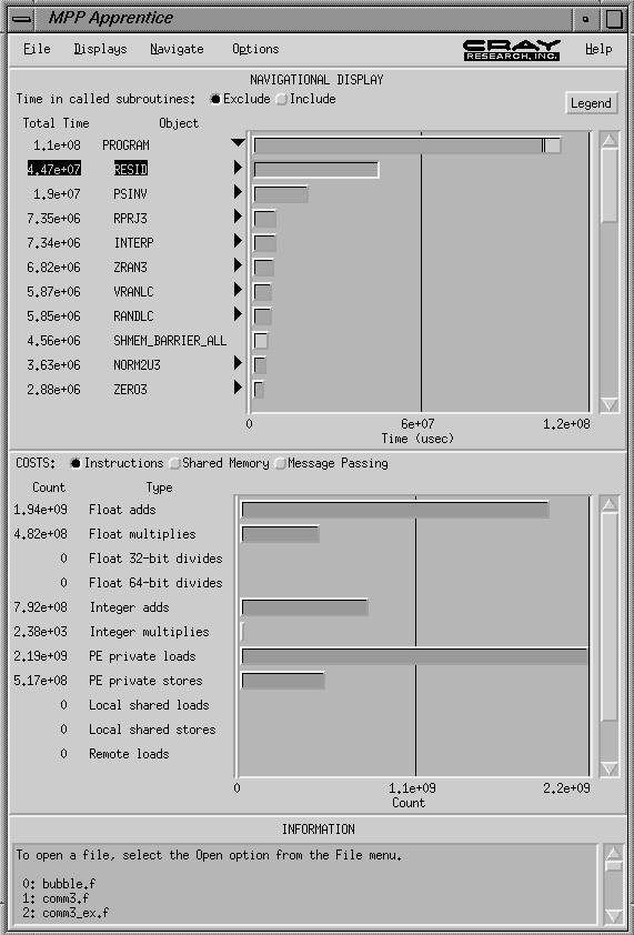
Apprentice initially displays the time spent in each routine. This time is broken down into time spent in parallel work, I/O time, overhead time, and called routine time. It also indicates time spent in uninstrumented sections for routine calls and i/o. Overhead time includes operations such as waiting on barriers. Apprentice also provides a breakdown of the costs for the routines. There are displays for three types of costs: basic instructions, shared-memory constructs and message-passing. The basic instructions include floating point and integer arithmetic operations as well as local and remote memory accesses. For the Craft/HPF programming model, Apprentice has the capability of reporting whether the memory accesses were to private or shared memory locations. The shared-memory construct costs show where time is spent in barriers and indicate the presence of critical regions. The message-passing costs indicate the time spent in calls to message-passing libraries. The libraries that Apprentice recognizes include SHMEM, PVM and MPI. Additionally, the Apprentice window provides a spot where messages from the tool to the user are displayed. These messages include items like explanations of errors. Apprentice is integrated with a language-sensitive source code browser that allows the user to easily find data structures and language constructs in the source to assist in analyzing the Apprentice information.
The user can drill down on any routine to see the same times and costs reported for sections of the routine. Because Apprentice inserts the instrumentation with some intelligence, the sections are tied to constructs such as DO loops or statements with line numbers corresponding to the source code. These statement and numbers are accurate even when high levels of compiler optimization are used (see Figure 10).
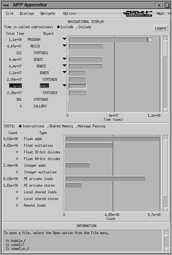
The interface allows the user to customize the displays from the preference menu. Examples of the items the user can control are the units used to display the various quantities reported, the method by which the routines are sorted, and whether context-sensitive help is used. These preferences may be captured for reuse when Apprentice is used the next time. The user has a great deal of control over the displays and can utilize peel-off windows to save various items of interest while continuing to pursue other options with the tool (see Figure 11).
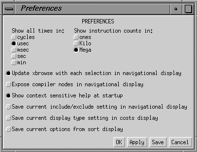
The "Observations" display of Apprentice provides a report for the whole program or for an individual routine which indicates the rates at which various instructions, such as floating point operations, are executing. The observations also include a detailed description as to where problem spots may be in the code. Examples of this include how much time is lost due to single instruction issue, and instruction and data cache misses. It can also indicate if significant amounts of time are spent in critical regions, which can result in excessive serialization. Additionally, it indicates the statements in a given routine where most time is spent and can do this even at high levels of compiler optimization (Figure 12).
Figure 12: Apprentice Observations window.
Users of debuggers on single processor machines and on highly parallel machines want debuggers that are reliable and that do not introduce any changes to the behavior of the code. In addition, they must be easy to use. "Ease-of-use" becomes more difficult to provide as the number of processes involved increases. The information for a large number of processes must be presented in a way that can be displayed on a typical workstation screen. Users need an easy way to direct the debugger to insert breakpoints at subgroups of processes and to specify whether all processors should stop whenever one meets a breakpoint. The debugger needs to present the current status of the entire program in a concise manner so that the user can easily determine what the program is doing. From this summary, the user can navigate to a specific processor or set of processors to obtain more detailed information.
The most popular parallel debugger used in the applications chapters is called TotalView. TotalView is a source level, multi-process debugger, capable of debugging running programs or to perform a post-mortum debug from a core file. It has both an X-Windows and a line-mode user interface. It supports symbolic debugging of the languages Fortran 90 , High Performance Fortran (HPF), C++, and C. As with most debuggers, TotalView has control functions to run, attach to, step, breakpoint, interrupt, and restart a process. It facilitates the examination and modification of variables, registers, areas of memory, and machine level instructions. Rather then dwelling on these standard debugger capabilities, however, the focus of what follows will address the TotalView features that are beneficial to the specific needs of MPP machines.
Perhaps the most crucial MPP capability that TotalView has is its ability to control thousands of processes coherently. The first place this is seen is in the TotalView main window (Figure 13). This window displays a summary of the processes being controlled by TotalView. It organizes the processes into process sets, where all processes that are in the same state (breakpointed, stopped, running, etc.) and on the same instruction are grouped and described with a single entry.
This technique greatly reduces the amount of data that needs to be displayed to, and absorbed by, the user. The user can "dive" (right mouse button click) on an entry to bring up a process set window detailing the contents of the set. A process set entry can also be expanded (or collapsed) to view the top of its call sequence.
While the TotalView main window provides a high level view of the processes being debugged, the TotalView process window (Figure 14) provides details specific to an individual process. There is initially a single process window with sliders that can scroll through each of the processes or jump directly to a desired process. Separate process windows can be created as desired.
Near the top of the process window is a status bar. The status bar displays the current process identifier (PID) and processor element (PE), as well as the PE's state. There is also a process set mode of either ALL or SINGLE. Whenever control commands are given to TotalView (for instance, continue, step) the command applies either to all of the processes in the set (ALL) or only to the specific process that the process window is displaying (SINGLE).
TotalView's breakpoints are configurable with respect to MPP processes. When setting a breakpoint in a process window, diving on the breakpoint (Figure 15) provides an opportunity to define the breakpoint to apply to a single process, or to all processes. Additionally, once the breakpoint is hit, all processes can be stopped, or only the breakpointed process.
TotalView has a number of features related to viewing data in an MPP environment. Both the Cray T3D and T3E are distributed memory machines. As such, each process has its own memory space that is not directly available to the others. To even display the value of any variables, TotalView must access the memory specific to the process currently being displayed in the process window. When the window is scrolled to a different process, new values must be fetched from the new memory space.
A common technique when programming MPP applications is to divvy up the processing of a large array among several processes. By default, an array is private, that is, each process will have a separate copy of the array that the other processes can not access directly. When TotalView displays a private array, the data object window (Figure 16) used to display the array has a slider to select the process from which the array is coming. Of course, many of the array elements may be invalid, since the selected process is not maintaining them. The elements that the selected process is responsible for are dependent on the design of the application.
With the aid of programming models such as Craft F77 and HPF it is possible to use shared arrays instead of private arrays. These models provide TotalView with more complete information regarding which processes are using which array elements. When TotalView displays a shared array, the data object window will not have a slider to select the process. Instead, the array elements are labeled with the process that they are local to and all of the elements will be valid.
One of the difficulties in developing applications dealing with large amounts of data is being able to "look" at and make sense of so much information. With MPP machines this is all the more true. While using TotalView to look at individual array elements is useful and essential, it may be too close a view of the data. TotalView can instead present a two-dimensional slice of the data as a color "picture." The user supplies a minimum and maximum value, a number of colors, and TotalView divides that range by the number of colors. In this way each value falls into a range and is mapped to the range's color. Each element of the array is then "painted" in its color to the rectangular picture. Values outside of the range are given a special color, as are floating point NAN values on IEEE units. This provides a coarse, high level picture of the data that can visually highlight data anomalies.
TotalView can also provide statistical summaries of the data. It will display the minimum, maximum, and sum of an array. Once again this can be useful in locating data anomalies.
Figure 13: TotalView Main Window
Figure 14: TotalView Process Window
Figure 15: TotalView Breakpoint Window
Figure 16: TotalView Data Object Window
Achieving peak performance on MPP systems depends both on how well an application scales across processors and on how close the performance of a portion executed on a single processor can come to the peak performance of that processor. Other sections of this chapter address scaling; indeed, the remaining chapters discuss how different applications are written to take advantage of many processors. The majority (ten of seventeen) of the applications discussed in this book were concerned with single-processor optimization. (See table in Section 8.) In this section, common techniques for getting the best performance for one processor are discussed. Single-processor optimization will vary depending on the exact characteristics of the processor, but the principles in this section, which apply explicitly to the Cray T3E system, will provide a good background. This section is purely introductory. For detailed assistance, the programmer should find the appropriate benchmarker's or programmer's guide to optimizing for a particular MPP computer system.
On the Cray T3E computer system, with its very strong network for interprocessor communication, the key to performance of a whole, well-parallelized application is typically optimizing for good performance on a single node. Substantial single-processor speedup is available from within high-level programming languages and from libraries. Additional performance can be obtained by hand optimization and assembly programming. In all cases, the goals of optimization are to use the processor's functional units at maximum capacity, to align data to take best advantage of the on-chip cache, and to understand and use any techniques available to mask the effects of having to load and store needed data that is not in cache. The goal, overall, is to hide the real time it takes to get data from memory to the processor's functional units and back again--the memory latency. Without attention to single-processor optimization, a programmer may obtain less than a tenth of the theoretical peak speed of the microprocessor. With considerable care, some optimized kernels can obtain up to two-thirds of peak.
Modern FORTRAN and, to a degree, C language compilers do quite a good job of keeping any processor's functional units as busy as possible, assuming the programmer exposes sufficient parallelism to the compiler. How to write good code for the compilers and how to take advantage of their capabilities is the subject of other texts and of compiler documentation. In short, a programmer must explicitly place sufficient work inside of loops to allow the functional units to amortize their startup time for an operation, must explicitly "unroll" inner loops with too little work or allow the compiler or libraries to do so, and must understand what operations and library calls inside loops prevent effective pipelining into the functional units and avoid, reposition, or modify them.
Using the FORTRAN 90 compiler on the Cray T3E system, a programmer can obtain considerable functional unit optimization by selecting the compiler options for general optimization (-O3 will do general optimization and allow calling vectorized versions of intrinsic functions like SIN and COS), for unrolling loops (-Ounroll2 causes the compiler to unroll loops, and -Ounroll1 directs the compiler to unroll loops if indicated via a compiler directive in the program), and for software pipelining (-Opipeline1 or -Opipeline2 will safely expose some additional independent operations to the functional units). In addition, the programmer may use compiler directives inside the program to indicate loop unrolling (!dir$ unroll n) or to tell the compiler that a loop is vectorizable (!dir$ ivdep). On many processors, including the Cray T3E processor, the floating-point divide is so very slow in loops that it is best replaced with multiplication by the reciprocal. Finally, highly optimized, but not always completely standards-compliant, library routines may be available to improve performance. On the Cray T3E system, for example, libmfastv and the unsupported benchlib may both be used, but programmers should take care to understand any possible side effects. The effects on performance of using the functional units effectively can be considerable, as stated above. Factors of three to eight speedup for certain loops can easily be obtained.
Compiler documentation and programmer's guides for particular systems will give the best detail on functional unit optimization for both the novice and experienced parallel programmers. The following example from the Cray T3E system shows how unrolling is done by hand, not unlike what a compiler would do. In addition, it demonstrates clearly that a compiler, with some minimal guidance, can attain better results than a programmer can do with substantial effort. Arrays A, B and C are each of size 256 and are stored consecutively so that all three arrays can reside in the Dcache at the same time. The loop is repeated many times to get a cache-resident performance figure:
	DO I = 1, 256
		A(I) = B(I) + 2.5 * C(I)
	ENDDO
When compiled with f90 -O3, without any unrolling, the loop's performance rate is about 53 MFlops. When compiled with f90 -O3,unroll2, which unrolls by 4, the performance improves to 155 MFlops. Manually unrolling the loop to help the compiler manage the functional unit dependencies, as follows, attains 177 MFlops:
	TEMP1 = 2.5*C(1)
	TEMP2 = 2.5*C(2)
	TEMP3 = 2.5*C(3)
	TEMP4 = 2.5*C(4)
	DO I = 1, 252, 4
		A(I) = B(I) + TEMP1
		TEMP1 = 2.5*C(I+4)
		A(I+1) = B(I+1) + TEMP2
		TEMP2 = 2.5*C(I+5)
		A(I+2) = B(I+2) + TEMP3
		TEMP3 = 2.5*C(I+6)
		A(I+3) = B(I+3) + TEMP4
		TEMP4 = 2.5*C(I+7)
	END DO
	A(I) = B(I) + TEMP1
	A(I+1) = B(I+1) + TEMP2
	A(I+2) = B(I+2) + TEMP3
	A(I+3) = B(I+3) + TEMP4
However, the easiest way to increase the functional unit parallelism is simply to unroll more deeply and let the compiler do the work. Adding the following directive before the original loop:
!DIR$ UNROLL 8
and recompiling with f90 -O3,unroll1, obtains the best performance of 181 MFlops.
The benefits of using optimization such as loop unrolling are discussed by a number of authors in the applications. In application chapter 1 (Table 1), the speedup obtained using different optimization procedures is shown. In application chapter 12, a dramatic speedup is cited for unrolling inner loops.
Data caches on the processor provide a first level to hide latency. Data in the caches can be moved to and from the processor in a few clock periods, whereas data in memory may take one or two orders of magnitude longer. On the Cray T3E processor, there is an 8KB primary data cache (Dcache), an 8KB instruction cache, and a 96 KB secondary cache (Scache) for both instructions and data. Within the cache, data is loaded and stored in "lines," of 32 bytes for Dcache and 64 bytes for Scache. Characteristics of the Scache help prevent cache thrashing, but the small sizes of the caches may require special attention of the Cray T3E programmer. On the Cray T3E-900 system, the Dcache latency is 2 clock periods, the Scache latency is 8-10 clock periods, and the memory latency is approximately 125 clock periods. Thus processing data not in the caches takes a great toll, since the processors are capable of performing two floating point operations per clock period.
As with functional unit optimization, compiler directives provide some cache optimization with little reprogramming. For example, both FORTRAN and C directives force data structures to be aligned on cache-line boundaries for the Cray T3E system and permit padding within common blocks to avoid some conflicts. Cache alignment assures that successive loads and stores from a data structure will not cause the cache to be flushed unnecessarily. From FORTRAN, the CACHE_ALIGN directive may be used as follows:
	REAL A(M,K), B(K,N), C(M,N)
	COMMON /ACOM/ C
CDIR$ CACHE_ALIGN A,B
CDIR$ CACHE_ALIGN /ACOM/
Similarly, in C, alignment is specified with a #Parma:
#Parma _CRI cache_align flags
int flags[4096];
Even with directives, the programmer may need to exercise some care in programming. In particular, it is important to understand what portions of arrays are used together in program sequences and then to ensure that the array segments and any other data used simultaneously resides in the cache to be accessed without flushing the cache. Finally, when the leading dimension of a cache-aligned array is a multiple of the cache-line size, columns are pulled into the cache on line boundaries. To ensure such alignment, it may be necessary to increase the leading dimensions of the arrays to a multiple of the cache-line size. However, the interplay of cache and buffering schemes in a particular MPP system may mean that choosing a good leading dimension depends on how the data is used.
The following example is adapted from a benchmarkers optimization [And97]of a finite difference kernel which has a small enough working data set (513) to benefit from optimization for the cache:
	REAL, DIMENSION(513,513) :: AA, DD, X, Y, RX, RY
	DO J = 2,N-1
		DO I = 2,N-1
			XX = X(I+1,J)-X(I-1,J)
			YX = Y(I+1,J)-Y(I-1,J)
			XY = X(I,J+1)-X(I,J-1)
			YY = Y(I,J+1)-Y(I,J-1)
			A = 0.25 * (XY*XY+YY*YY)
			B = 0.25* (XX*XX+YX*YX)
			C = 0.125 * (XX*XY+YX*YY)
			AA(I,J) = -B
			DD(I,J) = B+B+A*REL
			PXX = X(I+1,J)-2.*X(I,J)+X(I-1,J)
			QXX = Y(I+1,J)-2.*Y(I,J)+Y(I-1,J)
			PYY = X(I,J+1)-2.*X(I,J)+X(I,J-1)
			QYY = Y(I,J+1)-2.*Y(I,J)+Y(I,J-1)
			PXY = X(I+1,J+1)-X(I+1,J-1)-X(I-1,J+1)+X(I-1,J-1)
			QXY = Y(I+1,J+1)-Y(I+1,J-1)-Y(I-1,J+1)+Y(I-1,J-1)
			RX(I,J) = A*PXX+B*PYY-C*PXY
			RY(I,J) = A*QXX+B*QYY-C*QXY
		END DO
	END DO
The inner loop of this kernel has 47 floating point operations, 18 array reads and 4 array writes. The reads are of two 9-point stencils centered at X(I,J) and Y(I,J), and the writes consist of unit-stride stores to the independent arrays AA, DD, RX and RY. The two 9-point stencil array references should exhibit good temporal locality provided the three contiguous columns of X and Y fit simultaneously in the Scache. In addition, the writes to AA, DD, RX, and RY may not interfere with X and Y in the Scache. Since all six arrays are the same size and are accessed at the same rate, they will not interfere with each other if they do not conflict initially.
In the benchmarking example, [And97], to prevent a conflict, the arrays are placed in a cache-line aligned common block and padding arrays inserted between them to achieve the desired offsets modulo 4096. The leading dimension of the arrays is changed from 513 to 520 in order to make it a multiple of 8 words, the Scache line size. The modified Fortran is as follows:
	REAL, DIMENSION(520,513) :: AA, DD, X, Y, RX, RY
	PARAMETER (IPAD=3576)
	COMMON /ARRAYS/ X, P1(IPAD+520*3), Y, P2(IPAD+520*3), &
&	AA, P3(IPAD+128), DD, P4(IPAD+128), RX, P5(IPAD+128), RY
!DIR$ CACHE_ALIGN /ARRAYS/
	DO J = 2,N-1
		DO I = 2,N-1
			{Loop body omitted ...}
		END DO
	END DO
These changes improved the performance of the kernel by roughly a factor of two when compiled with f90 -O3,unroll2,pipeline2 on a Cray T3E-900 system. Such benefits have since been adopted into the compiler, making changes to the code more portable. For instance, using the compiler option "-a pad," and the cache align directive statement in the code without precomputing the optimum array and pad sizes yields almost the same improvement:
	REAL, DIMENSION(513,513) :: AA, DD, X, Y, RX, RY
	COMMON /ARRAYS/ X, Y,  AA, DD,  RX,  RY
!DIR$ CACHE_ALIGN /ARRAYS/
	DO J = 2,N-1
		DO I = 2,N-1
			{Loop body omitted ...}
		END DO
	END DO
To see the further potential benefits of cache-line alignment, consider the case of copying an 8-by-N array to another 8-by-N array [Ben97], in which both arrays have been deliberately misaligned so that each 8-element column spans two Scache lines, instead of one:
	INTEGER LDX, N
	PARAMETER (LDX=64, N=1000)
	REAL MBYTES, SECS, T1, T2
	REAL A(LDX,N), B(LDX,N)
	COMMON /AB/ BAD(4), A, B
!DIR$ CACHE_ALIGN /AB/
	DATA A / 64000*1.0 /
	CLKSPD = CLOCKTICK()
	T1 = RTC()
	CALL COPYAB( 8, N, A, LDX, B, LDX )
	T2 = RTC()
	MBYTES = 8.0*REAL( 16*N ) / 1.E+6
	SECS = (T2-T1)*CLKSPD
	WRITE(*,*) '8-BY-N BLOCK COPY = ', MBYTES/SECS,' MB/SEC'
	END
	SUBROUTINE COPYAB( M, N, A, LDA, B, LDB )
	INTEGER N, LDA, LDB
	REAL A(LDA,N), B(LDB,N)
	DO J = 1, N
		DO I = 1, M
			B(I,J) = A(I,J)
		END DO
	END DO
	RETURN
	END
In all of these computations, using a routine like CLOCKTICK, which returns the speed in seconds of one clock period in the microprocessor, is useful for comparing results on processors of different speeds:
#include <unistd.h>
float CLOCKTICK(void) {
	long sysconf(int request);
	float p;
	p = (float) sysconf(_SC_Cray_CPCYCLE); /* CPU cycle time in picoseconds */
	p = p * 1.0e-12;	 /* cycle time in seconds */
	return (p);
}
When compiled with f90 -O3,unroll2, the 8-by-N block matrix copy runs at 104 MB/sec, counting each byte copied once on the read and once on the write.
Now the arrays A and B are aligned on an 8-word Scache-line boundary by removing the array BAD in the common block declaration:
COMMON /AB/ A(LDX,N), B(LDX,N)
The performance improves by nearly a factor of two, to 195 MB/sec. However, using cacheable loads and stores leads to inefficient use of the caches in this example because only a small portion of the arrays A and B remain in cache on completion. E-register usage, described briefly below, would improve the performance.
Stream buffers on the Cray T3E node permit unit-stride or small-stride accesses to local memory to be streamed when an operation causes Scache misses for two consecutive 64-byte blocks of memory. There are six stream buffers on each node, and the hardware keeps track of eight cache misses, so non-contiguous misses may still cause streaming, and stream references may be interleaved. Optimizing for the stream buffers focuses on creating long patterns of unit-stride or small-stride access to memory to keep streaming active and grouping operations to limit memory references so that six or fewer streams can satisfy them.
Optimization guides for the Cray T3E system explain a number of techniques for using the stream buffers effectively, including:
A couple of examples from those guides will give a flavor for how using the stream buffers well can improve performance:
	SUBROUTINE FDTD(CAEX,CBEX,CAEY,CBEY,CAEZ,CBEZ,EX,EY,EZ,
&	HX,HY,HZ)
	REAL CAEX, CBEX, CAEY, CBEY, CAEZ, CBEZ
	REAL EX(129,129,128), EY(129,129,128), EZ(129,129,128)
	REAL HX(129,129,128), HY(129,129,128), HZ(129,129,128)
	DO J = 2, 127
		DO I = 2, 127
			DO K = 2, 127
				EX(K,I,J) =	CAEX*(EX(K,I,J) +
&					CBEX*(HZ(K,I,J) - HZ(K,I,J-1) +
&					HY(K,I,J) - HY(K-1,I,J)))
				EY(K,I,J) =	CAEY*(EY(K,I,J) +
&					CBEY*(HX(K-1,I,J) - HX(K,I,J) +
&					HZ(K,I-1,J) - HZ(K,I,J)))
				EZ(K,I,J) =	CAEZ*(EZ(K,I,J) +
&					CBEZ*(HX(K,I,J-1) - HX(K,I,J) +
&					HY(K,I,J) - HY(K,I-1,J)))
			END DO
		END DO
	END DO
	RETURN
	END
At first glance the six arrays seem an ideal fit for the six stream buffers. But because the loop accesses the well-separated columns j and j-1 of the arrays HX and HZ, there are at least eight input streams, three of which are also output streams. This loop is a good candidate for splitting because the trip counts are high, there are long sequences of unit stride references, and the arrays are large enough that they cannot already reside in the Scache. Just directing the compiler to split (-O3,split2) the innermost loop nets a 40% improvement. Splitting the loop manually may give different results.
An alternative strategy that works nearly as well is to condense several streams into a temporary vector as rewriting the above example shows:
	SUBROUTINE FDTD(CAEX,CBEX,CAEY,CBEY,CAEZ,CBEZ,EX,EY,EZ,
&	HX,HY,HZ)
	REAL EX(129,129,128), EY(129,129,128), EZ(129,129,128)
	REAL HX(129,129,128), HY(129,129,128), HZ(129,129,128)
	REAL TMP(3,128)
	DO J = 2, 127
		DO I = 2, 127
			DO K = 2, 126, 2
				TMP(1,K) = HZ(K,I,J) - HZ(K,I,J-1)
				TMP(2,K) = HX(K-1,I,J) - HX(K,I,J) +
&			HZ(K,I-1,J) - HZ(K,I,J)
				TMP(3,K) = HX(K,I,J-1) - HX(K,I,J)
				TMP(1,K+1) = HZ(K+1,I,J) - HZ(K+1,I,J-1)
				TMP(2,K+1) = HX(K,I,J) - HX(K+1,I,J) +
&			HZ(K+1,I-1,J) - HZ(K+1,I,J)
				TMP(3,K+1) = HX(K+1,I,J-1) - HX(K+1,I,J)
			END DO
			DO K = 2, 127
				EX(K,I,J) = CAEX*(EX(K,I,J) +
&			CBEX*(TMP(1,K) + HY(K,I,J) - HY(K-1,I,J)))
				EY(K,I,J) = CAEY*(EY(K,I,J) +
&			CBEY*(TMP(2,K)))
				EZ(K,I,J) = CAEZ*(EZ(K,I,J) +
&			CBEZ*(TMP(3,K) + HY(K,I,J) - HY(K,I-1,J)))
			END DO
		END DO
	END DO
	RETURN
	END
The first loop over k contains five streams, consisting of the array tmp and two columns each of HZ and HX. The second k loop also contains five streams: three for the arrays EX, EY, and EZ, one for HY, and one for TMP (which may still be in the cache). This version returns 57.6 MFlops. This is a lot more work than just splitting the loop, but it may be the only option if the inner loop variables all depend on each other.
Operations directly between the memory of any two PEs on the Cray T3E make use of special hardware components called E registers. These memory-mapped registers reside in noncached memory and provide a means for bypassing the cache when the data structure is such that use of the cache would be a hinderance. The E-registers, which are generally reserved for internal system use such as synchronization and communication with remote memory, can also play a critical role in helping applications scale well on many processors. They have a secondary use for local optimization, because they can assist in providing large-stride and gather/scatter operations very efficiently with respect to local memory, too. One can use the E-registers to obtain large blocks of data and for loads that would cause large amounts of data to be discarded if loaded into a cache-line. The E-registers can be used directly in a loop by specifying the CACHE_BYPASS directive. Their use may also be invoked by use of Shmem library and other special library routines. While it is beyond the scope of this section to give the detail necessary for using the E-registers, one example of a random gather will show the benefit to be gained:
!DIR$	CACHE_BYPASS A,X
	DO I = 1, NGATH
		X(I) = A(INDEX(I))
	END DO
Bypassing the cache and using the E-registers causes the data transfer rate on a Cray T3E-900 system to improve from 59 MB/s to 339 MB/s. Further improvement can be possible using special benchmarking library routines.
The E-registers are used by the compiler, external communications routines, and other libraries, and so the programmer needs to understand how to synchronize direct use of the registers with the other uses.
This section has given an idea of the techniques available to the applications programmer for automatic, semi-automatic and manual optimization for the single processor of an MPP system. As demonstrated in some of the examples, giving attention to single-processor performance can be well worth the effort. On the Cray T3E system, an experiment was performed using some of the NAS Kernel benchmarks which demonstrate characteristics of a NASA workload.
When the kernels were run unmodified and various options were chosen on the compiler command line, the overall performance of the set improved by a factor of four. Intrinsic function vectorization, common block padding, unrolling, software pipelining and linking with fast math intrinsic functions all contributed to the overall improvement, though some routines benefited more than others. One kernel improved by over a factor of six. From the experiment, the benchmarkers conclude that the compiler options -O3, unroll 2, pipeline2, -apad and loading the fast, but not completely IEEE-compliant, libfastmv should be selected for best automatic optimization.
Next, the benchmarkers examined each kernel in detail, modifying it as required. Many of the changes simply involved calling optimized library routines to perform the operations of the kernels. Sometimes, through pattern matching, the compiler is able to do this automatically, but not always. Compiler directives to align data in cache, use of the E-registers and cache-bypass, and rearranging array dimensions and splitting loops for better stream usage are some of the other techniques they used. In the end, they obtained, on average, another factor of three for the kernels, giving over a 6X average performance improvement in all. One kernel , which did not benefit much from the compiler-line options gained a factor of over six from hand-tuning.
The best overall combined improvement was a factor of twenty-one. And one kernel, a matrix multiplication, obtained over two-thirds the peak performance of the processor. These are impressive results, worth some effort, even keeping in mind that the performance of a kernel is often far superior to the average performance of a whole application.
In the industrial and scientific parallel computing environment, it is usually the case that a high end supercomputer has many users at all times. As an applications programmer, it is important to understand some of the issues associated with the scheduling of jobs on a parallel computer. These issues can help the user to both obtain maximum performance for a particular application and also understand the reasons why performance on a particular application may be significant less than expected in a multi-user environment.
For example, we consider in some detail the generations of schedulers developed for use on the multi-user and multi-program parallel environments at the Lawrence Livermore National Laboratory (LLNL) known as gang scheduling. Gang scheduling incorporates three principles: concurrent scheduling of each thread of a parallel program, space-sharing, and time-sharing. Space-sharing refers to the ability to concurrently execute different programs on the different processors. Most parallel computers provide only two of these components, resulting in significant loss of capability. Three generations of LLNL-developed gang schedulers have achieved excellent system utilization, good responsiveness, and effective parallel job execution on a variety of computer architectures. Gang scheduling provides parallel computers with capabilities ranging from general purpose through grand challenge computing.
Parallel computers are valuable resources from which one should expect a high level of system utilization. A high level of responsiveness is also required for the sake of program developers who execute many small programs. Interactive programs account for 67 percent of all jobs executed on LLNL's Cray T3D while consuming only 13 percent of all CPU cycles delivered. Peak interactive workloads reach 320 processors for a 25 percent over subscription rate, necessitating a time-sharing mechanism to provide good responsiveness. The remainder of resources are delivered to the larger and longer running batch jobs.
Most MPP systems provide concurrent scheduling of a parallel program's threads and space-sharing of resources. A time-sharing capability is normally lacking and processors allocated to a program are retained until that program's termination. This paradigm makes high system utilization and good responsiveness mutually incompatible. Given the high value of MPP systems, most are operated to provide high system utilization and limited responsiveness. Interactive work may be limited to a small subset of the processors and short execution times. Alternately, high priority batch queues may be constructed for programs having short execution times. Interactive and other high priority programs can not be initiated in a timely fashion during periods of high system utilization, precluding general purpose computing. Programs with high resource requirements must accumulate processors in a piecemeal fashion as other programs terminate, wasting those resources in the interim and reducing system utilization. Long running programs can prevent the execution of high priority or high resource requirement programs for extended periods. The lasting effect of scheduling a grand challenge class problem limits the system's ability to process them.
The addition of a time-sharing capability addresses these issues, with some relatively minor costs. Program preemption does incur some additional overhead, but higher overall system utilization may compensate for this. All running or preempted programs must have their storage requirements simultaneously satisfied. Preempted programs must also vacate memory for other programs. As with non-parallel computers, the increased system capability and effective capacity provided by time-sharing should warrant the expense of additional storage. It should be noted that grand challenge class problems typically utilize most of the available real memory. The true cost of performing a context switch in this environment may be tens of seconds and result in terabytes of data moving between real memory and disk (virtual memory). This I/O normally prevents the instantaneous responsiveness available for small problem sizes.
Most symmetric multiprocessor (SMP) systems do provide both time-sharing and space-sharing, but lack a mechanism for concurrent scheduling of a parallel program's threads of execution. Concurrent scheduling of a program's threads has been shown to improve the efficiency of both the individual parallel programs and the system [Dus96, SoWe95]. Concurrent scheduling is essential not only within a single SMP, but across a cluster in order harness the compute power available and address grand challenge class problems.
The objective of gang scheduling is to achieve a high level of system utilization and responsiveness on parallel computing platforms in multiprogrammed environments. The concurrent execution of a parallel program's threads can be viewed as essential for any scheduler implementation. Sustained system utilization rates over 90 percent are practical for SMP architectures and can be extended into MPP domain. While maximizing the responsiveness for all programs might be attractive, our design objective was somewhat more refined: to provide high responsiveness only for programs in which the expected benefit outweighs the high context switch times described earlier. The responsiveness requirement for interactive programs is far more critical than that of batch programs. The LLNL gang scheduler was therefore designed to maximize responsiveness for interactive and other high priority work. Responsiveness for batch and lower priority work was not a significant concern.
The LLNL gang scheduler was initially developed for the BBN TC2000 system in 1991 [GoWo95]. It underwent substantial modification for use on the Cray T3D in 1996 [FeJe97, Jet96]. Its third generation was developed for clusters of DIGITAL Alpha computers in 1997 [Jet97, Jet98]. While the LLNL gang scheduler has evolved during this period and significant system specific differences exist, many original design features remain.
One significant design feature is the existence of several job classes, each with different scheduling characteristics. These classes permit the scheduler to provide high responsiveness only to programs for which the additional overhead will provide real benefit, primarily in cases where a user is waiting at a terminal for the response. The classes also provide for a variety of throughput rates depending upon programmatic considerations. The following job classes are supported: express jobs have been deemed by management to be mission critical and are given rapid response and optimal throughput, interactive jobs require rapid response time and very good throughput during working hours, debug jobs require rapid response time during working hours but can not be preempted on the Cray T3D due to the debugger's design, production jobs do not require rapid response, but should receive good throughput at night and on weekends, benchmark jobs do not require rapid response, but can not be preempted once execution begins, standby jobs have low priority and are suitable for absorbing otherwise idle compute resources.
Each parallel program has a job class associated with it. The default classes are production for batch jobs, debug for TotalView debugger initiated jobs, and interactive for other jobs directly initiated from a user terminal. Jobs can be placed in the express class only by the system administrator. Benchmark and standby classes can be specified by the user at program initiation time. Each job class has a variety of associated parameters, the most significant being the class's relative priority. All LLNL gang scheduling parameters can be altered in real time to provide different scheduling characteristics at different times. For example, LLNL systems are configured to provide high responsiveness and interactivity during working hours. Throughput is emphasized at night and on weekends.
Resource management is provided by other systems that can alter a program's nice value in response to a user's or group's resource consumption rate diverging from the target consumption rate. Nice value changes can result in a program being reclassified to or from the standby job class.
The parallel program to be scheduled must register its resource and scheduling requirements with the appropriate gang scheduler daemon at initiation time. No user applications modifications were necessary on either the BBN and Cray systems since it was possible to substitute LLNL developed software for the vendors' parallel program initiation software. Initiating parallel programs on DIGITAL computers can be as simple as executing a fork system call, which is impossible to capture outside of the operating system. Therefore, DIGITAL parallel programs must be modified to register their resource requirements and each process must explicitly register as a component of the program. This typically requires the addition of one function call in the user application and makes use of an LLNL developed library to issue remote procedure calls to the gang scheduler daemon.
From the point a parallel program has been registered, the gang scheduler daemons decide which resources are to be allocated to it and when. While executing, each program has the perception of dedicated resources. A program's throughput is primarily dependent upon overall system load and relative priority of the program's job class.
The cost of performing a context switch for typical LLNL parallel programs is quite substantial. On architectures supporting virtual memory, paging essentially removes the entire memory image of one program in order to load that of another program. The time to perform this paging raises effective context switch time into the tens of seconds range (for large programs, into the range of minutes). In order to amortize this substantial context switch time, they should occur at infrequent intervals. The key to providing good responsiveness with infrequent context switching is the prioritized job classes. Rather than providing time-sharing of resources among all executable programs, resources are specifically targeted to the highest priority work through what may be better described as a preemption scheme. For example, an interactive class job may preempt a production class job. The preempted production class job will not resume execution until no higher priority work can be allocated those resources. If multiple programs at the same job class priority contend for the same resources, those programs may time-share the resources. The net effect is a high utilization and low overhead system with good responsiveness.
The first generation LLNL gang scheduler was developed in 1991 for the BBN TC2000 "butterfly" [GoWo95], a 126-processor computer shared-memory architecture. The TC2000 originally supported only space-sharing of resources. The gang scheduler reserved all resources at system startup, and controlled all resource scheduling from that time . User programs required no modification to take advantage of the gang scheduler, but did need to load with a modified parallel job initiation library. Rather than securing resources directly from the operating system, this modified library was allocated resources by the gang scheduler daemon. Each time-slice lasted ten seconds with decisions made as to resource allocation at each time-slice boundary. Context switches were initiated through concurrent transmission of signals to all threads of a parallel program.
The second generation LLNL gang scheduler required major modification for the Cray T3D system in 1996 [FeJe97, Jet96]. The LLNL Cray T3D system had 256 processors, each with 64 megabytes or DRAM. Only space-sharing of resources was originally permitted on the Cray T3D. In 1996 Cray Research added a capability to save a parallel program's context to disk and later restore it to memory. The implementation also permitted the restoration of a program to different processors, which permitted workload rebalancing and significant improvement in performance. Parallel programs on the Cray T3D are initiated through a vendor supplied program. LLNL developed a "wrapper" for this program to register its resource requirements with the gang scheduler daemon at initiation time and receive a specific resource allocation. The gang scheduler daemon performs context switches by issuing system calls. Scheduling decisions are made whenever a program is initiated or terminated, completion of writing a program's state to disk, and on a periodic basis. This event driven scheduler provides for better responsiveness than would be possible with fixed period time-slices.
The third and latest generation LLNL gang scheduler supports DIGITAL SMP systems with the Digital Unix operating system [Jet97, Jet98]. While Digital Unix does provide for space-sharing and time-sharing, it fails to coordinate scheduling of a parallel program's threads. This is addressed through program and thread registration with the gang scheduler daemon and DIGITAL's class scheduler. Rather than providing a mechanism to assign specific processors to specific processes, the class scheduler resembles a very fine-grained fair-share scheduler. Real-time changes to the class scheduler parameters control which programs are running or preempted. The operating system seeks to take advantage of an active cache, tending to keep a given thread on a specific processor. The net effect is very similar to true gang scheduling. To coordinate scheduling across multiple SMP computers, it was necessary to revert to fixed time-slice periods (currently configured at 30 seconds). If appropriate, newly initiated programs may begin execution prior to a time-slice boundary. Programs with particularly large memory requirements may be scheduled to run in multiple consecutive time-slices to limit paging. Each computer has its own gang scheduler daemon which is capable of operating independently for greater fault tolerance. Programs spanning multiple computers require coordinated scheduling by multiple gang scheduler daemons. Remote procedure calls are used to establish time-slice allocations across multiple computers. Tickets representing these resources are associated with programs through their lifetime.
While the LLNL gang scheduler's basic design calls for resource allocation to the highest priority programs, high context switch times necessitated some additional consideration. One additional parameter associated with each job class on the Cray T3D implementation is a do not disturb factor. Once a program is allocated resources, it is guaranteed those resources for some period before preemption occurs. This time period is computed by multiplying the number of processors the program is allocated by the do not disturb factor. This parameter limits the impact context switches may have upon overall system throughput. Multiple programs with identical job class priorities will context switch periodically, but memory thrashing will be avoided.
Another parameter associated with each job class is a maximum wait time. A program waiting longer than the maximum wait time for its resource allocation will have those resources reserved for it. Multiple programs of equal or lower priority will be preempted after satisfying their do not disturb requirement. This insures that programs with high resource requirement can be allocated those resources in a timely fashion.
To ensure that high responsiveness is provided to non-parallel programs on DIGITAL SMP systems, a parameter is provided to specify a minimum number of processors to be reserved for them. These processors will be available to execute system daemons and non-parallel user programs in a timely fashion.
One other parameter will be noted, a maximum workload. Once the system's workload reaches this level, newly initiated programs will be queued for execution but not scheduled. Programs which have already begun execution will continue. The purpose of this parameter is to prevent oversubscription of storage space, especially swap space. The maximum workload is specified in terms of processor count.
The introduction of the LLNL gang scheduler on the Cray T3D permitted substantial reconfiguration of the machine. Rather than reserving a substantial number of processors for interactive use during working hours, the batch system was permitted to completely allocate all processors at all times. Interactive work is allocated resources on an as needed basis. While the median time required to begin execution of interactive programs has increased slightly, the worst case has been dramatically reduced by time-sharing resources during periods of extreme load. Substantially longer running programs were permitted to execute and freed from the constraint of only executing during weekend hours.
The overall Cray T3D system utilization improved substantially after deployment of a gang scheduler. This improvement in utilization can be largely attributed to the reconfiguration described above. Weekly Cray T3D processor utilization frequently exceeded 96 percent. About two percent of CPU time is lost to incomplete resource allocation due to a workload incapable of utilizing every processor. Context switch time also reduces CPU utilization by about two percent since the CPU is idle during the entire time a program's state is moved between memory and rotating storage. In benchmarks run against an early version of the LLNL gang scheduler for the Cray T3D, throughput of interactive work increased by 21 percent without reduction in overall system throughput.
Responsiveness may be quantified by slowdown or the amount by which a program's actual execution time exceeds its execution time in a dedicated environment. Since the LLNL design only ventures to provide a high level of responsiveness to interactive programs, responsiveness for batch jobs will not be considered. The aggregate interactive workload slowdown on the Cray T3D during a 20 day period of high utilization was 18 percent, which is viewed quite favorably. Further investigation shows a great deal of variation in slowdown. Most longer running interactive jobs enjoy slowdowns of only a few percent. Interactive jobs executed during the daytime typically begin execution within 30 seconds and continue without preempted until termination. Interactive jobs executed during late night and early morning hours experienced slowdowns as high as 1371 (a one second job delayed for about 23 minutes). However the computer is configured for high utilization and batch job execution during these hours, so high slowdowns are not unexpected.
Gang scheduling on the DIGITAL systems demonstrates significant improvement in performance for tightly coupled parallel programs, especially at high levels of parallelism and heavily loaded computers. One factor in performance improvement is a fast reduction in spin-wait time at synchronization points. Spin-waiting keeps a processor polling for an event rather than relinquishing the processors. While this technique maximizes program throughput, it can result in substantial waste of compute resources. Another important factor is a reduction in the cache refresh overhead, which is provided by the long slice times (configured at 30 seconds). While executing with gang scheduling, the program effectively has dedicated memory and processor resources. Figure 17 shows the effect of gang scheduling on the performance of a Gaussian elimination benchmark. This computer used for the benchmark was being concurrently used by about 14 other runable threads, the normal state of affairs for our interactive oriented computers during normal work hours.
Figure 17: Gaussian elimination benchmark performance on DIGITAL Computer
No degradation in overall system responsiveness or utilization has been noted. This is in part due to the DIGITAL class scheduler's ability to reallocate otherwise idle resources should the parallel program wait for some external event. A wide range of parallel programs demonstrate five to 100 percent speedup in response to concurrent scheduling of threads. Figure 18 shows the performance of a parallel program and the computer system executing it. The left window shows overall system performance. The windows on the right show performance of the parallel application. CPU and memory use information is plotted at each time-slice boundary to aid in tuning both the computer system and application program.
Figure 18: Display of gang scheduling two parallel programs on DIGITAL computer
The addition of a time-sharing capability to MPP computers can substantially improve both the system's capability and effective capacity. Good responsiveness provides the user with an effective program development environment and the means to rapidly execute short programs. The ability to initiate resource intensive problems upon demand, without the piecemeal accumulation of resources, increases overall system utilization. Long running programs can also be initiated as desired without preventing the reallocation of those resources at a later time for high priority or resource intensive problems.
SMP systems benefit by the concurrent scheduling of a parallel program's threads, particularly across multiple computers. This extends the range of SMP capabilities beyond general purpose computing to that of grand challenge class problems.
The applications chapters in this book cover a wide variety of sub-fields. In the process of parallelizing a major applications code, it is often the case that one must call upon a variety of numerical methods and techniques. This is because for a complex "real" application code, there are many processes working simultaneously often on different time scales. Thus in grouping the applications chapters in the book, we have not attempted to partition them out based on numerical schemes and parallel computing techniques. Rather they are categorized based on the essential length scale of the physical phenomena modeled. On the largest scale, we have meso- to macro-scale environmental modeling. Next down from this in primary physical scale-length, we have a category that broadly covers fluid dynamics. Although plasmas can be classified as fluids and can also have length scales greater than a typical Navier-Stokes fluid, they often involve processes on shorter time-scales that allow for the interaction of the electrons and ions in the plasma. Thus we use this classification next down in our rough break-down and have a section for applied plasma dynamics. Continuing to get smaller in physical phenomena, we categorized certain of the chapters as materials design and modeling. Here, the applications codes tend to deal with primarily particle and/or molecular interactions in contrast to the more global behavior of the plasma category. Finally, an additional set of applications dealt primarily with data analysis applications rather than a problem characterized by physical length scales, so we have grouped these applications accordingly.
To assist the reader with finding information pertinent to the creation of a new parallel application code, we also cross-reference the articles based on certain parallel techniques and numerical methods that are exploited and carefully explained in the chapters. For this classification scheme, we number the applications codes from 1-17 based on their order of appearance in the table of contents. Thus (1) refers to "Ocean Modeling and Visualization on a Massively Parallel Computer." In the following table, we generate a list of the projects and some of the important techniques.
Table 1
: Classification of the applications based on the numerical methods, parallel computing issues, and programming model used or discussed.
Methods, Issues, and Models Addressed in the Applications |
|||||||||||||||||
|
Application Code Number |
1 |
2 |
3 |
4 |
5 |
6 |
7 |
8 |
9 |
10 |
11 |
12 |
13 |
14 |
15 |
16 |
17 |
|
|
|||||||||||||||||
|
Numerical Methods |
|
|
|
|
|
|
|
|
|
|
|
|
|
|
|
|
|
|
Iterative Matrix Methods/Sparse Matrices |
x |
x |
x |
|
|
x |
|
|
|
|
|
x |
|
x |
|
|
|
|
Eigenvalues, Eigenvectors |
|
|
|
|
|
|
|
|
|
x |
|
x |
|
|
|
|
|
|
Discrete and Fourier Transforms |
|
|
|
|
|
|
|
|
|
x |
x |
x |
x |
|
x |
|
|
|
Finite Difference Methods |
x |
x |
x |
|
|
x |
|
|
x |
x |
|
|
|
|
|
|
|
|
Finite Element Methods |
|
|
|
|
|
|
|
|
|
|
|
|
|
x |
|
|
|
|
Finite Volume Methods |
|
|
|
x |
x |
x |
|
|
|
|
|
|
|
|
|
|
|
|
Mesh Generation and Refinement |
|
|
|
|
|
|
x |
|
|
|
|
|
x |
|
|
|
|
|
Domain Decomposition including Multi-Grid |
|
x |
x |
x |
|
x |
x |
|
|
x |
|
|
|
|
|
|
x |
|
Particle in Cell/Particle Tracking |
|
|
|
|
x |
|
x |
|
x |
|
|
|
|
|
|
|
|
|
Integral Equations, Integrals |
|
|
|
|
x |
|
x |
|
|
x |
|
x |
|
x |
|
|
|
|
Optimization, local |
|
|
|
|
|
|
|
|
|
|
|
|
|
|
x |
x |
|
|
Parallel Random Field Generation |
|
|
|
|
|
x |
|
|
|
|
|
|
|
|
|
|
|
|
|
1 |
2 |
3 |
4 |
5 |
6 |
7 |
8 |
9 |
10 |
11 |
12 |
13 |
14 |
15 |
16 |
17 |
|
Parallel Computing Issues |
|
|
|
|
|
|
|
|
|
|
|
|
|
|
|
|
|
|
Single Processor Optimization |
x |
|
x |
|
x |
|
x |
|
|
x |
x |
x |
x |
x |
x |
|
|
|
Parallel I/O |
|
|
|
|
|
|
x |
|
|
x |
x |
x |
|
x |
x |
|
|
|
Load Balancing |
|
|
|
|
x |
|
x |
x |
x |
x |
x |
x |
x |
x |
x |
x |
|
|
Performance Comparison on Various Architectures |
|
x |
|
|
|
x |
x |
|
x |
|
x |
x |
|
|
x |
x |
|
|
Use of Parallel Tools Discussed |
x |
x |
|
x |
|
|
x |
|
|
|
|
|
|
|
x |
|
|
|
Networking, realtime |
|
|
|
|
|
|
|
|
|
|
|
|
|
|
x |
|
|
|
Processing, realtime |
|
|
|
|
|
|
|
|
|
|
|
|
|
|
x |
|
x |
|
Scheduling, interactive |
|
|
|
|
|
|
|
|
|
|
|
|
|
|
x |
|
|
|
|
1 |
2 |
3 |
4 |
5 |
6 |
7 |
8 |
9 |
10 |
11 |
12 |
13 |
14 |
15 |
16 |
17 |
|
Programming Models |
|
|
|
|
|
|
|
|
|
|
|
|
|
|
|
|
|
|
MPI |
x |
x |
x |
x |
|
|
x |
x |
|
x |
|
x |
x |
|
|
|
|
|
PVM |
|
|
x |
x |
x |
|
|
|
|
|
|
|
|
|
x |
x |
|
|
SHMEM |
x |
x |
x |
|
|
|
x |
x |
|
x |
x |
|
x |
x |
|
|
x |
|
HPF/CRAFT |
|
|
x |
|
|
|
x |
|
|
|
|
|
|
x |
|
|
|
|
Other Models and Preprocessors |
|
x |
x |
|
|
x |
|
|
|
|
|
|
|
|
x |
|
|
|
Task farming |
|
|
|
|
|
|
|
|
|
|
|
|
|
|
x |
x |
|
|
Other Issues |
|
|
|
|
|
|
|
|
|
|
|
|
|
|
|
|
|
|
Graphics and Volume Rendering |
x |
|
|
|
|
|
x |
|
|
x |
|
|
|
|
x |
|
|
|
Parallel Software Libraries |
x |
|
x |
|
|
|
x |
|
|
|
x |
|
|
|
x |
|
|
|
Dynamic programming |
|
|
|
|
|
|
|
|
|
|
|
|
|
|
|
x |
|
[And97] E. Anderson, J. Brooks, C. Grassl, S. Scott, "Performance of the Cray T3E Multiprocessor," Proceedings SC97, San Jose.
[Ben97] E. Anderson, J. Brooks, and T. Hewitt, "The Benchmarker's Guide to Single-processor Optimization for Cray T3E Systems," Cray Research, a Silicon Graphics Company, Publication, 1997.
[Beo97]Thomas Sterling, "How to build a Beowulf: Assembling, Programming, and Using a Clustered PC Do-it-yourself Supercomputer, Supercomputing '97.
[Bro97] Eugene D. Brooks III and Karen Warren, "A Study of Performance on SMP and Distributed Memory Architectures Using a Shared Memory Programming Model," In Proceedings of the 1997 ACM/IEEE SC97 Conference. [BSP] "BSPlib: The BSP Programming Library," Jonathan M. D. Hill, Bill McColl, Dan C. Stefanescu, Mark W. Goudreau, Kevin Lang, Satish B. Rao, Torsten Suel, Thanasis Tsantilas, and Rob Bisseling. Technical report PRG-TR-29-9, Oxford University Computing Laboratory, May 1997. [CaJe95] William Carson and Jess Draper, "AC for the T3D," Supercomputing Research Center Institute for Defense Analyses, Technical Report SRC-TR-95-141, February 1995.
[Cha92] B. Chapman, P. Mehrotra, H. Zima, "Programming in Vienna Fortran," Scientific Programming, Fall 1992. [Cul93] David C. Culler, Andrea Dusseau, Seth Copen Goldstein, Arvind Krishnamurthy, Steven Lumetta, Thorsten von Eicken and Katherine Yelick, "Parallel Programming in Split-C," Proceedings of the Supercomputing Conference, Portland, 1993. [Cul98] David Culler, Jaswinder Pal Singh with Anoop Gupta, "Parallel Computer Architecture, A Hardware/Software Approach," Morgan Kaufmann, 1998 [Cri89] "Cray Y-MP, Cray X-MP EA, and Cray X-MP Multitasking Programmer's Manual", SR-0222F, Cray Research Publication, 1989. [Don97] Jack J. Dongarra, Subhash Saini, Erich Strohmaier, and Patrick H. Worley, "Performance Evaluation of Parallel Applications: Measurement, Modeling, and Analysis," Supercomputing '97, San Jose.
[Dus96] A. C. Dusseau, R. H. Arpaci and D. E. Culler, "Effective Distributed Scheduling of Parallel Workloads." ACM SIGMETRICS `96 Conference on the Measurement and Modeling of Computer Systems, 1996. [FeJe97] D. G. Feitelson and M. A. Jette, "Improved Utilization and Responsiveness with Gang Scheduling," IPPS '97 Workshop on Job Scheduling Strategies for Parallel Processing, Apr 1997, http://www-lc.llnl.gov/global_access/dctg/gang/gang.sspp.ps.
[Fin72] M.J. Flynn, "Some computer organizations and their effectiveness," IEEE Transactions on Computing, 21:948-960, 1972.
[Fos96] Ian Foster, David R. Kohr Jr., Rakesh Krishnaiyer, Alok Choudhary, "Double Standards: Bringing Task Parallelism to HPF Via the Message Passing Interface," Proceedings of the 1996 Supercomputing ACM/IEEE Supercomputing Conference. [Fox91] G. Fox, S. Hiranandani, K. Kennedy, C. Keolbel, U. Kremer, C. Tseng, and M. Wu, "Fortran D Language Specification," Department of Computer Science, Rice University. COMPTR90079, March 1991. [GoWo95] B. Gorda and R. Wolski, "Timesharing massively parallel machines," International Conference on Parallel Processing, Volume II, Aug 1995, pp. 214-217. [Gro96] Wm Gropp, Ewing Lusk, Anthony Skjellum, "Using MPI, Portable Parallel Programming with The Message-Passing Interface," MIT Press, Cambridge, MA, 1996. [HPF]"High Performance Fortran Language Specification," Version 2.0, January 1997, High Performance Fortran Forum. [Jet96] M. Jette, D. Storch and E. Yim, "Gang Scheduler - Timesharing the Cray T3D," Cray User Group, Mar 1996, pp. 247-252, http://www-lc.llnl.gov/global_access/dctg/gang/gang.sched.html. [Jet97] M. Jette, "Performance Characteristics of Gang Scheduling in Multiprogrammed Environments," Supercomputing 97, Nov 1997. [Jet98] M. Jette, "Expanding Symmetric Multiprocessor Capability Through Gang Scheduling," IPPS '98 Workshop on Job Scheduling Strategies for Parallel Processing, Apr 1998. [Koe93] C. Koelbel, D. Loveman, R. Schreiber, G. Steele, and M. Zosel, "The High Performance Fortran Handbook," MIT Press, Cambridge, MA, 1993. [Meh97] P. Mehrotra, J. Van Rosendal, H.Zima, "High Performance Fortran: History, Status and Future," TR 97-8 Sept 1997, University of Vienna, Institute for Software Technology and Parallel Systems [MeRe96] Michael Metcalf and John Reid, "Fortran 90/95 Explained," Oxford University Press, 1996.
[MPI1] "A Message-Passing Interface Standard," Message Passing Interface Forum, May, 1994. University of Tennessee, Knoxville, Tennessee.
[MPI2] "Extensions to the Message-Passing Interface," Message Passing Interface Forum, July 1997, University of Tennessee, Knoxville, Tennessee.
[NPB] The NAS Parallel
Benchmarks home pages.
http://www.nas.nasa.gov
[NuSt97] R. Numrich and J. Steidel, "Simple Parallel Extensions to Fortran 90," Proceedings of the Eighth SIAM Conference on Parallel Processing for Scientific Computing, 1997, SIAM Activity Group on Supercomputing. [ReNu98] J. Reid and R. Numrich, Rutherford Appleton Laboratory, "Formal and Informal Definitions of fmm," In preparation, 1998. [SHMEM] "SHMEM, Application Programmer's Library Reference Manual," Cray Research Inc. Publication SR-2165.
[Sni96] Marc Snir, Steve W.Otto, Steven Huss-Lederman, David W. Walker, Jack Dongarra,"MPI, The Complete Reference," MIT Press, Cambridge, MA, 1996. [SoWe95] P. G. Sobalvarro and W. E. Weihl, "Demand-based Coscheduling of Parallel Jobs on Multiprogrammed Multiprocessors." IPPS '95 Parallel Job Scheduling Workshop, Apr 1995.
[SP2] T. Agerwala, J. L. Martin, J. H. Mirza, D. C. Sadler, D. M. Dias, and M. Snir, "SP2 System Architecture," IBM Systems Journal, Reprint Order No. G321-5563, 1995.
[StDo96] Aad J. van der Steen and Jack J. Dongarra, "Overview of Recent Supercomputers," 10 Feb 1996, (Sixth Edition).
http://www.crpc.rice.edu/NHSEreview.
BSP Home Page: http://www.bsp-worldwide.org LLNL Gang Scheduling Home Page: http://www-lc.llnl.gov/global_access/dctg/gang/ HPF Home Page: http://www.crpc.rice.edu/HPFF/home.html PVM Home Page: http://www.epm.ornl.gov/pvm/pvm_home.html MPI Home Page: http://www.mcs.anl.gov/mpi/ URLs
OpenMP Home Page: http://www.openmp.org
1. Figures 6 and 7 and the data flow example are from the "Cray T3E Fortran Optimization Guide, SG-2518" and are used by permission.