maxdimsystems - determination of maximum dimensional subsystems of systems of PDE

maxdimsystems( system , maxdimvars )

maxdimsystems( system , maxdimvars , options )

Parameters

system - list or set of ODE or PDE (may contain inequations)

maxdimvars - list of the dependent variables used for the dimension count

options - (optional) sequence of options to control the behavior of maxdimsystems

• The default output of maxdimsystems (modulo *** below) consists of the set of cases having maximal dimension in maxdimvars , where each member has the form:

• Solved is a list of the PDE which are in solved form with respect to their highest derivative (with respect to the given ranking of derivatives), Constraint is a list of the PDEs in the classvars (any dependent variables not in maxdimvars ) which are nonlinear in their leading derivatives, Pivots is a list of the inequations in the classvars and/or maxdimvars, and dimension is the maximal degree of arbitrariness in maxdimvars (i.e. the number of arbitrary constants on which maxdimvars depends).
• *** The result is valid provided that the Constraint and Pivots equations have a solution, and also that maxdimvars do not occur in the constraint equations. The user must check the first condition algebraically (e.g. see Groebner[gsolve] , and possibly diffalg ). If the maxdimvars are present in the pivots, then the returned system will have lower dimension that indicated, and must be handled manually.

• Each of the cases is in rifsimp form (a generalization of Gauss normal form to systems of PDE) and also contains a system of differential equations and inequations in the classvars characterizing the case. In the same way that the Gauss normal form is determined by a ordering of variables, rifsimp form is determined by a ranking of derivatives.
• The default ranking is determined by maxdimvars . It can be inferred by the application of checkrank , and always ranks the classvars and their derivatives lower than all maxdimvars .
• The maximal cases can be determined in many applications where a complete analysis of all cases is not possible. These cases are often the most interesting, with the richest properties, when compared to the relatively uninteresting (but often difficult to compute) lower dimensional cases.
• The options for maxdimsystems consist of the output option (described below), and a subset of those for rifsimp , the main subroutine used by maxdimsystems. Of the subset of rifsimp options available, two that are often used are indep which specifies the independent variables, ezcriteria which controls the flow of equations from a fast (ultra-hog) setting (that can readily lead to memory explosion but sometimes faster calculations), to a conservative (one equation at a time) setting that can overcome some expression swell problems. The complete list is given by:

• Many rifsimp options are not supported by maxdimsystems as their use could produce misleading results. For example, the rifsimp option ctl=time , places a time limit on rifsimp case computations, and hence could cause maxdimsystems to miss the maximal case if it takes too long to compute. Conversely, specification of other options are not supported as they must have a specific value for the maxdimsystems command to function properly (for example, casesplit must always be on). Other unsupported rifsimp options include itl , stl , nopiv , unsolved , pivsub , store , storeall , spawn , spoly , and casecount .

• output = type

• The output type can either be set (default) or rif . Note that set output is easier to read and manipulate, but cannot be used with the caseplot visualization tool. The rif output can be used with caseplot , but the output is somewhat more complicated, and is described in rifsimp[output] . Note that for the class of problems that maxdimsystems simplifies, many of the outputs from rifsimp described in the output page ( such as DiffConstraint and UnSolve ) will never be present in the output.

• The maxdimsystems command allows a subset of the rankings available for rifsimp . Specifically those rankings that are controlled by a partition of the dependent variables in maxdimvars , and those available by the order of the independent variables in indep . See rifsimp[ranking] and checkrank for an explanation of how to specify rankings based on these options.
• The application of caseplot to the rif -form output of maxdimsystems with the second argument given as the maxdimvars displays the tree of maximal cases and their dimensions, also indicating which branches of the tree have less than maximal dimension.
• Note that maxdimsystems is essentially a simplified version of the rifsimp interface that also has the ability to automatically determine the maximum finite dimensional cases or all infinite dimensional cases for a classification ODE/PDE system. If the dimension of the solution space is known, multiple conditions on the dimension of the solution space are needed, or much finer control of the computation is desired, then rifsimp could be used with the mindim option described in rifsimp[cases] .
• References:

> with(Rif):

Algebraic systems can be examined with maxdimsystems

> maxdimsystems([ u - a*v = 0, u - c*v = 0], [u,v]);

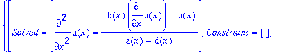
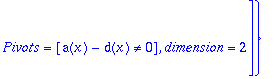
In the below example, inequations are given in the Pivots list, and the dimension is 2

> maxdimsystems([ (a(x)-d(x))*diff(u(x),x,x) +
b(x)*diff(u(x),x) + u(x) = 0],
[u]);

This next example has a constraint on the classvars present in the result

> maxdimsystems([diff(u(x,y),x) - f(x,y)*u(x,y) = 0,
diff(u(x,y),y) - g(x,y)*u(x,y) = 0,
f(x,y)^3 - 1 = 0], [u]);

In each of the above examples maxdimsystems picked out the maximum dimensional case. This is in contrast to rifsimp , with its casesplit option, which obtains all cases.

For the second example, computation with rifsimp using casesplit gives 2-d, 1-d and 0-d cases, of which the 2-d case is the maximal case from the above example.

> ans := rifsimp([ (a(x)-d(x))*diff(u(x),x,x) +
b(x)*diff(u(x),x) + u(x) = 0],
[u], casesplit);

from which the caseplot with initial data counts could be viewed by issuing the command:

> caseplot(ans,[u]);

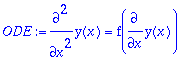
One example of practical use of maxdimsystems is the determination of the forms of f(y') (where f(y') is not identically zero) for which the ode y''=f(y') has the maximum dimension.

> ODE:=diff(diff(y(x),x),x)=f(diff(y(x),x));

> symeq:=[DEtools[odepde](ODE, [xi(x,y),eta(x,y)])];

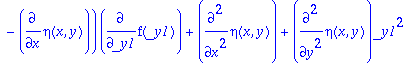
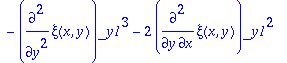
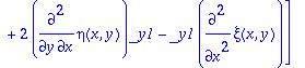
where the above symeq is an overdetermined system of PDE in the infinitesimal symmetries xi(x,y),eta(x,y) .

So we compute the maximum dimensional case which, is not displayed as it is quite large:

> t1 := time():
msys:= maxdimsystems([op(symeq),f(_y1)<>0],[xi,eta]):
time()-t1;

> nops(msys);

> length(msys[1]);

> msys[1][4];

> remove(has,rhs(msys[1][1]),[xi,eta]);

from which we see that we have one case, of dimension 8, and it occurs when the displayed ODE in f(_y1) is satisfied. This classical result is also explored in the ISSAC Proc. article listed in the references (the primary reference for this command).

The timing above should be compared to the rifsimp full case analysis that takes significantly longer, and has a great number of lower dimensional cases:

> t2 := time():
rsys:= rifsimp([op(symeq),f(_y1)<>0],[xi,eta],'casesplit'):
time()-t2;

> rsys['casecount'];

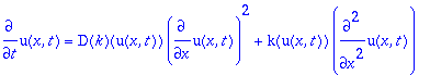
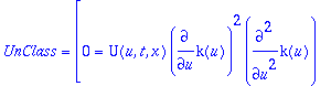
Consider the nonlinear Heat equation

> diff(u(x,t),t) = diff( k(u(x,t))*diff(u(x,t),x), x);

The overdetermined system for it's symmetries X,T,U is given by

> sys:= [
-2*diff(T(u,t,x),x),
diff(diff(U(u,t,x),u),u)-2*diff(diff(X(u,t,x),u),x)
+U(u,t,x)*diff(diff(k(u),u),u)/k(u)+1/k(u)
*diff(k(u),u)*diff(U(u,t,x),u)-U(u,t,x)/k(u)^2
*diff(k(u),u)^2,
1/k(u)*diff(X(u,t,x),u)*diff(k(u),u)
-diff(diff(X(u,t,x),u),u),
diff(diff(U(u,t,x),x),x)-1/k(u)*diff(U(u,t,x),t),
1/k(u)*diff(T(u,t,x),t)+U(u,t,x)/k(u)^2*diff(k(u),u)
-diff(diff(T(u,t,x),x),x)-2/k(u)*diff(X(u,t,x),x),
-diff(diff(X(u,t,x),x),x)+2*diff(diff(U(u,t,x),u),x)
+1/k(u)*diff(X(u,t,x),t)+2*diff(k(u),u)/k(u)
*diff(U(u,t,x),x),
-2*diff(k(u),u)/k(u)*diff(T(u,t,x),x)-2/k(u)
*diff(X(u,t,x),u)-2*diff(diff(T(u,t,x),u),x),
-1/k(u)*diff(k(u),u)*diff(T(u,t,x),u)
-diff(diff(T(u,t,x),u),u),
-2*diff(T(u,t,x),u)]:

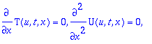
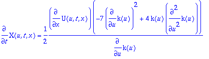
At the same time as determining maximum dimensional cases, one can request, through a partitioning of the maxdimvars , that the dependent variables be ranked in a specific manner. To always isolate derivatives of U(u,t,x) in terms of the other dependent variables, one could specify maxdimvars=[[U],[X,T]] . For this problem we would obtain

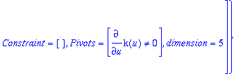
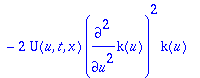
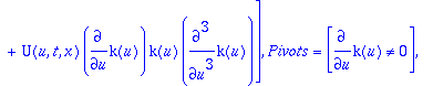
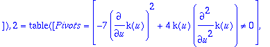
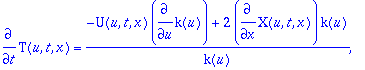
> maxdimsystems([op(sys),diff(k(u),u)<>0],[[U],[X,T]]);

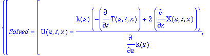
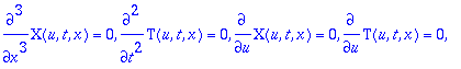
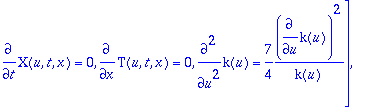
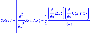
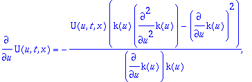
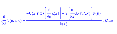
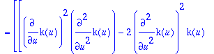
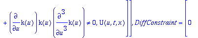
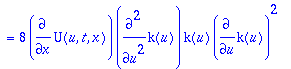
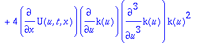
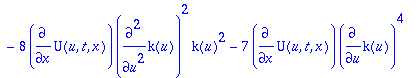
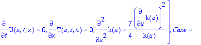
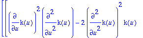
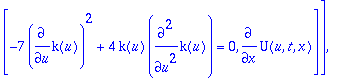
Alternatively we could try to obtain PDE only in U(u,t,x) and the classifying function k(u) by an elimination ranking:

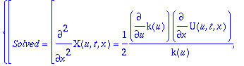
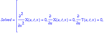
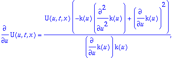
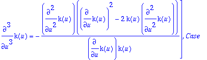
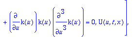
> maxdimsystems([op(sys),diff(k(u),u)<>0],[[X,T],[U]]);

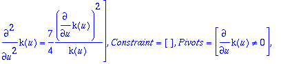
where you can see from the above that we have three PDE for U(u,t,x) alone (which can be quite easily solved for U(u,t,x) in terms of a function that is linear in x with coefficients as integrals in u depending on k(u) ).

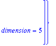
Both computations show that maximal group is of dimension 5, and occurs when k(u) satisfies k'' = 7/4 (k')^2/k . This is a known result (see the Bluman/Kumei reference).

In determining how a specific ranking will be used in a system, one should consult the checkrank help page.

The final example demonstrates how to find near-maximal cases, and how to obtain rif -style output. Say we want all cases having dimension 4 or greater, and we want rifsimp output (so we can display the information in a case plot). This can be done as follows:

> rifans:=maxdimsystems([op(sys),diff(k(u),u)<>0],[X,T,U],
mindim=4, output=rif);

All cases where the initial data was smaller than the bound are tagged with a status of "free count fell below mindim". This calculation can then be displayed in a caseplot with the command:

> caseplot(rifans,[X,T,U]);

Rif , rifsimp , initialdata , checkrank , rifsimp[adv_options] , rifsimp[cases] , rifsimp[nonlinear] , rifsimp[options] , rifsimp[output] , rifsimp[overview] , rifsimp[ranking]