rifsimp[output] - description of algorithm output

• The output of the rifsimp command is a table. A number of possible table formats (or entries) may or may not be present as they depend on specific options. The format changes from a table containing the simplified system to a nested table when casesplit is activated.
• Single Case

• Here are examples of status messages:

• Of the above, only the "object too large" message actually indicates an error.

• To summarize, if the input system is fully linear in all indeterminates (including unknown constants), then only the Solved entry will be present. If the system is (and remains) linear in its leading indeterminates throughout the calculation, but has indeterminate expressions in the leading coefficients, then Solved , Pivots , and Case will be present. If equations that are nonlinear in their leading indeterminates result during a calculation, then Constraint will also be present. If the status entry is present, then not all information for the case will be given.

• If mindim is used, then the dimension entry will be set to the dimension of the linear part of the system for the case when status is not set, and an upper bound for the dimension of the case if the count fell below the minimum dimension requirement.

• Multiple Cases

• For multiple cases (using the casesplit option), numbered entries appear in the output table, each of which is itself a table of the form described above.
• For example, if a calculation resulted in 10 cases, the output table would have entries '1=...',..., '10=...', where each of these entries is itself a table that contains Solved , Pivots , Case , or other entries from the single case description.
• In addition to the numbered tables is the entry casecount , which gives a count of the number of cases explored. Cases that rejected for reasons other than inconsistency will have the Case entry assigned, in addition to the status entry. Inconsistent cases, for multiple case solutions, are removed automatically.

• So what is the difference between Pivots and Case ?

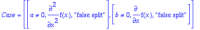
• The Pivots entry contains the inequations for the given case in simplified form with respect to the output system. The Case entry is a list with elements of the form [assumption,leading derivative] or [assumption,leading derivative,"false split"] . It describes the actual decision made for the case split in unsimplified form (i.e. as it was encountered in the algorithm). The assumption will be of the form expr<>0 or expr=0 , where expr depends on the dependent variables, derivatives and/or constants of the problem. The leading derivative is the indeterminate the algorithm was isolating that required the assumption . If the third "false split" entry is present, then it was later discovered that one branch of the split is entirely inconsistent, so the actual splitting was a false split ting, as the displayed assumption is always true with respect to the rest of the system. For example, if the algorithm were to split on an equation of the form a*diff(f(y),y)+f(y)=0 , the Case entries that correspond to this case split are [a<>0,diff(f(y),y)] , and [a=0,diff(f(y),y)] . If it was found later in the algorithm that a=0 leads to a contradiction, then the Case entry would be given by [a<>0,diff(f(y),y),"false split"] .
• Note that when faclimit or factoring are used (of which factoring is turned on by default), it is possible to introduce a splitting that does not isolate a specific derivative. When this occurs, the case entry will be of the form [assumption,"faclimit"] or [assumption,"factor"] .
• Occasionally both the Case and Pivots entries contain the same information, but it should be understood that they represent different things.

• Important

> with(Rif):

As a first example, we take the overdetermined system of two equations in one dependent variable f(x) , and two constants a and b .

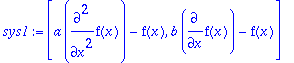
> sys1:=[a*diff(f(x),x,x)-f(x),b*diff(f(x),x)-f(x)];

Call rifsimp for a single case only (the default).

> ans1:=rifsimp(sys1);

We see that under the given assumptions for the form of a and b (from Pivots ), the only solution is given as f(x)=0 (from Solved ). Now, run the system in multiple case mode using casesplit .

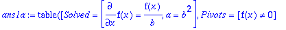
> ans1m:=rifsimp(sys1,casesplit);

We see that we have four cases:

> ans1m[casecount];

All cases except 2 have f(x)=0 .

Looking at case 2 in detail, we see that under the constraint a = b^2 (from Solved ) and b <> 0 from Pivots , the solution to the system will be given by the remaining ODE in f(x) (in Solved ). Note here that the constraint on the constants a and b , together with the assumption b <> 0 , imply that a <> 0 , so this constraint is not present in the Pivots entry due to simplification. It is still present in the Case entry because Case describes the decisions made in the algorithm, not their simplified result. Also, case 4 has no Pivots entry. This is because no assumptions of the form expression <> 0 were used for this case.

One could look at the caseplot with the command:

> caseplot(ans1m);

As a final demonstration involving this system, suppose that we are only interested in nontrivial cases where f(x) is not identically zero. We can simply include this assumption in the input system, and rifsimp will take it into account.

> ans1a:=rifsimp([op(sys1),f(x)<>0],casesplit);

We see that the answer is returned in a single case with two false split Case entries. This means the computation discovered that the a=0 and b=0 cases lead to contradictions, so the entries in the Case list are labelled as false split s, and the alternatives for the binary case splittings (cases with a=0 or b=0 ) are not present.

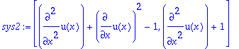
For the next example, we have a simple inconsistent system:

> sys2:=[diff(u(x),x,x)+diff(u(x),x)^2-1,diff(u(x),x,x)+1];

> rifsimp(sys2);

So there is no solution u(x) to the above system of equations.

The next example demonstrates the UnSolve list, while also warning about leaving indeterminates in unsolved form.

> sys3:=[diff(f(x),x)*(diff(g(x),x)-g(x))+f(x)^2,diff(g(x),x)-g(x)];

So we run rifsimp , but only solve for f(x) , leaving g(x) in unsolved form. Unfortunately, the resulting system is inconsistent, but this is not recognized because equations containing only g(x) are left unsolved. As discussed earlier in the page, these equations come out in the UnSolve list.

> rifsimp(sys3,[f],unsolved);

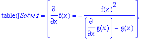
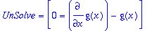
When equations are present in the UnSolve list, they must be manually examined.

Here is a nonlinear example.

> sys4:=[diff(f(x),x,x)+f(x),diff(f(x),x)^2-f(x)^2];

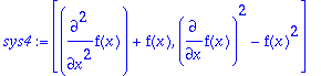
By default rifsimp spawns the nonlinear equation to obtain a leading linear equation, and performs any required simplifications. The end result gives the following output:

> rifsimp(sys4,casesplit);

We have only one consistent case. Attempting to perform this calculation with the spawn=false option gives the following:

> rifsimp(sys4,casesplit,spawn=false);

So it is clear that by disabling spawning, the system is not in fully simplified form (as indicated by the presence of the DiffConstraint entry), and we do not obtain full information about the system.

caseplot , rifsimp , rifsimp[adv_options] , rifsimp[cases] , rifsimp[nonlinear] , rifsimp[options]