


Next: Ising for language
Up: The Ising Model
Previous: Computational implementations
The Ising Model can be further refactored to model the dynamics of what we
call lexical attenuation in natural language.
Our model describes a possible history of the dynamics of a
meta-vocable. This meta-vocable is a statistical representation of all
vocables.
As in the standard model we use spin states to represent vocables on a
two dimensional lattice. We also use a Maxwellian demon lattice to
apply a local level of activity - the frequency of use - for
each constituents. In addition, we introduce the concept of attenuation and we use it as a statistical bias. It is similar to degeneracy in that it can be introduced as a feature of a two-dimensional Ising
model but with one difference: Usually a particular degeneracy value is
assigned homogeneously to each spin. In our case we introduce a
gradient of attenuation, that is, spins are assigned an
increasing number of potential attenuated states, illustrated as
a gradient. We will describe this process in detail a little later.
We use three Cartesian grids for our language model. The first grid
represents the two dimensional lattice that hosts spins. These spins
represent a set of instances or occurrences of one meta-vocable. A
black (or dark) pixel for a constituent represents a functional state of
the vocable while a blue (or light) pixel represents a lexical
state. Figure 6.4 illustrates a typical representation of that grid.
Notice the white line that travels the grid. This line highlights the
ratio between functional (dark pixel) and lexical (light pixel) for
all rows.
Figure 6.4:
Vocable (spin) grid. Vocables can be in 1
of 2 states; light is lexical while dark is
functional. The white line indicate the ratio
of light to dark for every row.
|
|
A second grid represents the local potential for attenuation. A
gradient from black to white describes the state of attenuation each
meta-vocable can achieve. The changing levels of attenuation can be
thought of as actual real time-line (versus simulation time) in the
lifespan of a vocable. Early instances are found in the dark areas of
the gradient while later instances are found in the light ones (see
figure 6.5)
Figure 6.5:
Attenuation grid. The different shades
represent degrees of attenuation; in this
case constituents can be attenuated up
to a 7 to 1 ratio.
|
|
This gradient affects the critical point at which a first-order phase
transition can occur within each area for each degeneracy.
For our physicist audience, let us remember that, given a Hamiltonian
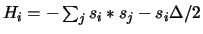 ,
the field value is
,
the field value is  (flipping a spin changes the energy by
  if spin values
are +1/-1), and attenuation is
if spin values
are +1/-1), and attenuation is  .
Because
changes along the length of the attenuation grid, we observe
(figure 6.6) that the critical point (green or dash line) is pushed
inwards as the level of attenuation augments.
.
Because
changes along the length of the attenuation grid, we observe
(figure 6.6) that the critical point (green or dash line) is pushed
inwards as the level of attenuation augments.
Figure 6.6:
This graph illustrates how the critical point (green or thick lines) at
which a first-order phase transition occurs moves inwards for
constituents ranging from 1 state of degeneracy to 3 states of
degeneracy. The x's indicate the state of constituents. Those
with 3 states of attenuation have become functionalized because
the activity level is past their critical point. The other constituents
remain lexical because their respective critical points have not been
reached.
|
|
Consider a simulation where there are mixed attenuated states for
constituents. The attenuation gradient is up to three states.
No state of attenuation is represented as black while attenuated states
from one to three is represented respectively as dark, medium
and light grey (as shown in figure 6.6). The
Meanfield solutions in figure 6.6 illustrates that
some attenuated constituents
remain lexical - x at the top of the curve - at a sub-critical level of
activity. Once the level of activity in the system
reaches the critical point of state change for particular states of attenuation,
constituents become functional -
x on the bottom curve. In this graph we illustrate the critical
points at which constituents will become functionalized.
Notice that only constituents that have
three states of attenuation have become functionalized because
their critical point has been reached.
As in the standard Ising model, we also use a bias that favours a particular
state energetically. Lexical vocables tend to stay lexical for reasons
energetically similar to the reasons why ice tends to remain in its
solid state until environmental constraints are such that a liquid
state becomes favoured. This feature, however, is not
graphically represented.
A third grid, corresponding to the Maxwellian demon grid, illustrates
an activity rate. The energy driving attenuation is the
physical effort expended in the actual uses of the vocables in speech.
The temperature variable used in the standard Ising model finds its
equivalent in the activity variable of our model. As the activity level is increased, the likelyhood for vocables - spins - to
become attenuated will also increase. Augmenting the activity value represents an increase in the use of vocables within a
linguistic community. In the real world, linguistic activity
increases with a growing number of linguistic participants in a
population; however, since our model has a finite population -
constituents, it is solely the frequency of use of a vocable that
defines the activity variable. For example, given a system
where there are only two linguistic participants, we can expect that
some vocables can become very attenuated by the mere fact of overuse.
Consider the case of technical language used by
small groups of people in the context of developing new technologies.
As the use of such vocables becomes attenuated, we lose our capacity
to say what it specifically means; we think that technical jargon is a product
of similar dynamics. Figure 6.7 illustrates local variances in the activity
levels of each constituent.
Figure 6.7:
Activity grid. This is a "Maxwell" demon
grid. A random level activity is assigned to every vocable constituent in the
system. The overall average is the activity in the system. It is equivalent
to the level of linguistic activity that can
occur in a population of language users.
|
|
Each spin site has a local activity value
assigned to it. In the application to language, a high activity
value at a spin site can be thought of as representing extensive use
of that vocable by a single user. The underlying theory suggests that
higher usage eventually entails a higher rate of attenuation. So a
low distribution of activity in the system can be taken to represent
comparative lexical richness.
Next: Ising for language
Up: The Ising Model
Previous: Computational implementations
Thalie Prevost
2003-12-24
![\includegraphics[scale=0.70]{spingrid}](img13.gif)
![\includegraphics[scale=0.70]{attenuationgrid}](img14.gif)
![\includegraphics[scale=0.60]{attenuationgraph}](img19.gif)
![\includegraphics[scale=0.70]{maxwellgrid}](img20.gif)